3.5 质粒综合实战

本页目录

本页准备
使用有来源的序列
组合独立图层
阅读各注释层
有意选择显示位点
理解目录和标签的限制
应用到自己的数据
完成后检查
保存本页结果
完整示例：pETDuet-1 密集质粒图

用随包 pUC19 DNA 完成一张可阅读的质粒图：注释、引物和酶切分别成层，显示选择与完整结果分开保存。

本页准备

在新的 R 会话中先运行下方代码，再按页面顺序继续。配色和排版是可选的显示设置，输入只选择需要的列。

准备代码 · 在本页运行一次

代码library(ggchord)
feature_palette <- c(
  CDS = "#993366", promoter = "#31849B", rep_origin = "#F1E51D",
  primer_bind = "#A020F0", misc_feature = "#A6ACB3", protein_bind = "#31849B"
)

library(ggchord)
doc_background <- "#FFFCF5"
identity_palette <- c("#303B71", "#36537D", "#269B82", "#A5D52C", "#ECEB31")
identity_values <- c(0, 0.5, 0.8, 0.9, 1)
identity_breaks <- c(0, 50, 80, 90, 100)
doc_legend_theme <- theme(
  legend.title = element_text(size = 13, face = "bold"),
  legend.text = element_text(size = 11),
  legend.key.width = unit(9, "mm"), legend.key.height = unit(5, "mm"),
  legend.spacing.x = unit(9, "mm"), legend.spacing.y = unit(7, "mm"),
  legend.margin = margin(l = 4, r = 4, unit = "mm")
)
sequence_guide <- guide_ggchord_legend(nrow = 1, theme = doc_legend_theme)
strand_guide <- guide_ggchord_legend(
  nrow = 1, override.aes = list(strand = c("+", "-")), theme = doc_legend_theme
)
identity_guide <- guide_ggchord_colourbar(
  position = "left", direction = "vertical",
  theme = theme(
    legend.key.height = unit(75, "mm"), legend.key.width = unit(5, "mm"),
    legend.title = element_text(size = 13, face = "bold"),
    legend.text = element_text(size = 11), legend.margin = margin(r = 7, unit = "mm")
  )
)
doc_theme <- theme_ggchord_publication(
  axis.text = element_text(size = 11),
  axis.text.check.overlap = TRUE
) +
  theme(
    legend.position = "bottom",
    legend.title = element_text(size = 13, face = "bold"),
    legend.text = element_text(size = 11),
    legend.key.width = unit(9, "mm"), legend.key.height = unit(5, "mm"),
    legend.spacing.x = unit(9, "mm"), legend.spacing.y = unit(7, "mm"),
    legend.box.spacing = unit(6, "mm"),
    plot.background = element_rect(fill = doc_background, colour = NA),
    panel.background = element_blank(),
    plot.title = element_text(face = "bold", size = 18),
    plot.subtitle = element_text(size = 10, colour = "#5C625A"),
    plot.margin = margin(14, 18, 14, 18)
  )
doc_axis <- function(coordinates = "relative") {
  scale_seq_position_continuous(
    coordinates = coordinates, n.breaks = 3, minor_breaks = NULL,
    labels = function(x) format(x, scientific = FALSE, big.mark = ",", trim = TRUE)
  )
}

其中定义了本例使用的配色。

使用有来源的序列

随包 plasmid_example_pUC19 原样来自仓库 examples/plasmid/pUC19.fna，不会为显示修改碱基或序列标识。本流程使用包中有来源记录的识别目录，不需要网络请求，也不为图形伪造实验测量值。

代码library(dplyr)
data(plasmid_example_pUC19)
plasmid_seq <- plasmid_example_pUC19 |>
  select(accver, length)
plasmid_feature_source <- find_common_features(plasmid_example_pUC19)
# Dedicated primer layers already show bindings; avoid duplicate primer annotations.
plasmid_features <- plasmid_feature_source |>
  filter(type != "primer_bind") |>
  select(accver, start, end, strand, type, anno)
plasmid_primers <- find_primer_bindings(plasmid_example_pUC19, set = "universal")
plasmid_sites <- find_restriction_sites(plasmid_example_pUC19)
display_sites <- filter_restriction_sites(plasmid_sites, enzymes = c("EcoRI", "BamHI", "HindIII"))
primer_names <- primer_catalog(set = "universal")

先查看 plasmid_features、plasmid_primers 与 display_sites，区分完整搜索与显示选择。

组合独立图层

下面按骨架、注释、标签、引物和酶切的顺序添加图层。注释与标签共享同一个 Position；每个图层只读取自己的数据。

代码plasmid_position <- position_feature_stack(spacing = .10, base_position = position_plasmid())
p_plasmid <- ggchord(seq_data = plasmid_seq) +
  geom_seq(seq_style = "double") +
  geom_feature_plasmid(aes(feature_fill = type), data = plasmid_features, position = plasmid_position) +
  geom_feature_label_repel(
    data = plasmid_features, position = plasmid_position,
    size = 4
  ) +
  geom_primer(data = plasmid_primers, colour = "#A020F0") +
  geom_primer_label_repel(data = plasmid_primers, colour = "#A020F0", max_overlaps = 0, size = 3) +
  geom_restriction_site(data = display_sites, colour = "#29364B", label_size = 3, leader = "radial") +
  geom_seq_center_label() +
  scale_feature_fill_manual(values = feature_palette) +
  scale_seq_position_continuous() +
  coord_circular(rotation = 90) +
  theme_ggchord_plasmid() +
  theme(
    legend.title = element_text(size = 13, face = "bold"),
    legend.text = element_text(size = 11),
    legend.spacing.x = unit(9, "mm"), legend.spacing.y = unit(7, "mm"),
    plot.background = element_rect(fill = doc_background, colour = NA),
    panel.background = element_blank()
  )
p_plasmid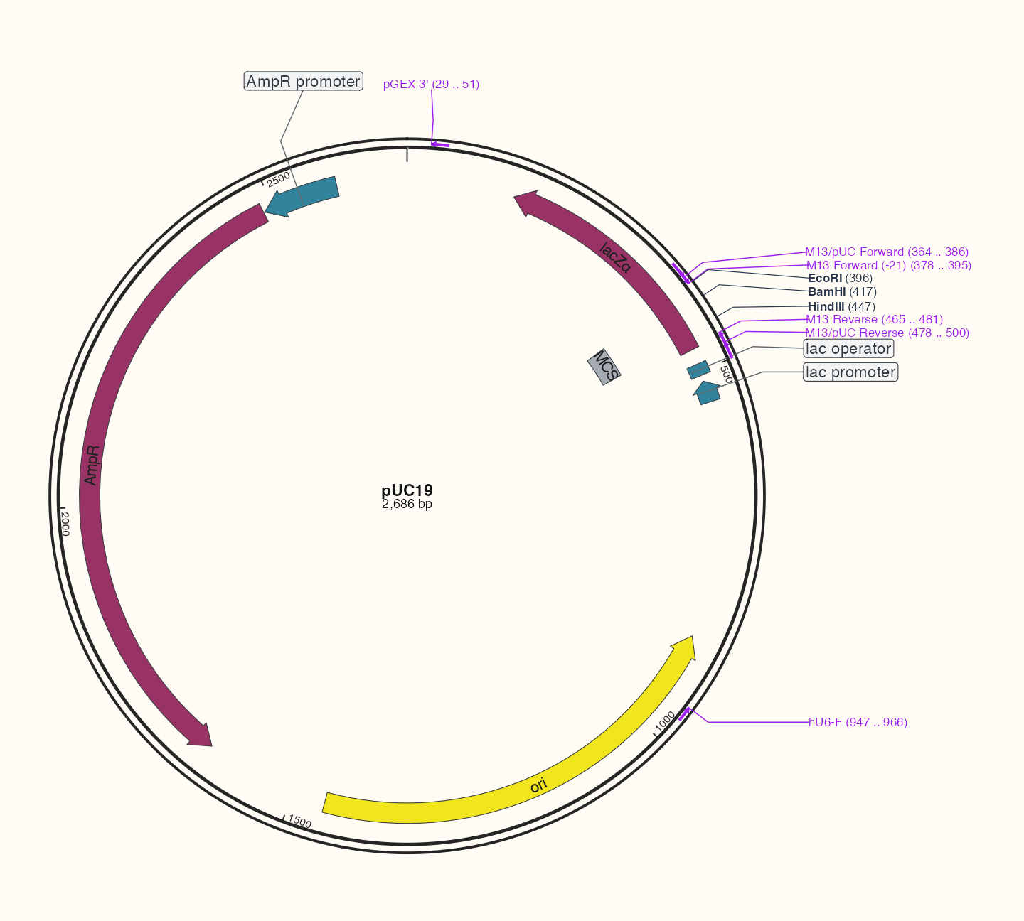

项目	结果
完整序列长度（bp）	2686
注释记录数	7
精确引物命中记录数	6
酶条目匹配记录数（非独立位置数）	49845
选定显示的酶切记录数	3

混合的圈外标签按锚点顺序共同排版，包括少量酶切标签与引物共存的情况。本例使用质粒专用主题和默认 feature 适配；默认先尝试内部文字，再使用相邻或外侧位置。不要通过不断缩小文字或强制手动偏移掩盖交叉；请在相同导出尺寸下检查。

原始注释保留在 plasmid_feature_source。显示表去掉 primer_bind 注释，交由独立引物层表达，避免重复；注释层只接收几何、类型和注释文字。

阅读各注释层

双线骨架建立单条圆形序列，通用注释使用 plasmid 预设和显式 stacking Position，标签共享该 Position。引物弧线表达结合范围，酶切短线表达切割/显示位置，中心标签给出序列名称和长度。裁剪或筛选显示不改变完整序列的酶位点计数。

有意选择显示位点

find_restriction_sites() 返回全部匹配。本图明确选择 EcoRI、BamHI 与 HindIII，使局部酶切簇保持可读；plasmid_sites 保留完整搜索结果。只有完整输入序列精确匹配参考时， reference 筛选才使用已保存的参考显示集合。其他任务可选 unique、six_plus 或明确酶名。绘图前检查 display_sites 及甲基化/来源列。参考集合是显示选择，不表示未知样本的生物学状态已经确定。

理解目录和标签的限制

primer_names 展示目录条目。本例精确搜索 universal 目录，参考引物注释与精确寡核苷酸搜索有不同来源。近似蛋白注释识别遵循识别专题的限制，不验证生物学功能或引物实验。文字可以移位、在显式字号下限内缩小或隐藏。应保留几何并在最终尺寸检查导出标签原因，而不是要求每条注释必须显示文字。

应用到自己的数据

将输入替换成有明确名称的 DNA 序列，先检查搜索结果再添加几何层。已有整理注释时，直接提供注释表，无需再次运行识别。堆叠与形状说明几何，标签说明适配，输出说明设备与尺寸。

geom_primer_label_repel(side = "inside") 将引物引出标签保留在骨架内侧，包括同时存在外侧酶切及注释标签时。0.16.6 已修复此行为； v0.16.5 可能将请求内侧的标签移到外侧。外侧默认布局和原始坐标不变。

内侧酶切标签继续保留内侧几何，导出 annotation registry 现在也正确记录内侧；早期版本将这些诊断行误标为外侧资源。

完整内侧场景仍可能出现长引物文字与其他 feature 区域交叠；默认 max_overlaps = Inf 不认证跨 feature 图层的零交叠。空间不足时优先使用默认外侧，或通过 show_location = FALSE 缩短显示文字，并在最终尺寸检查结果。

完成后检查

从中心的名称与长度开始，沿骨架读位置，再读类别色、箭头方向和外侧标签。核对 display_sites 的酶名；删减显示不会改变 plasmid_sites。

继续：放置和调整标签 →

保存本页结果

在工作目录中保存刚刚创建的图；预览时使用相同宽高。

代码ggsave("pUC19-map.png", p_plasmid, width = 10, height = 9, units = "in", dpi = 144)

完整示例：pETDuet-1 密集质粒图

先用上面的 pUC19 掌握图层，再用 pETDuet-1 展示复杂注释。以下来自随包真实序列、常见特征与参考引物表；酶切输入保留 commercial_all 中唯一的六碱基及以上识别位点，不把筛选后的图误称为全部酶的所有切点。

代码library(ggchord)
library(dplyr)
data(plasmid_example_pETDuet_1)
show_plasmid <- plasmid_example_pETDuet_1 |>
  select(accver, length)
show_plasmid_features <- find_common_features(plasmid_example_pETDuet_1)
show_plasmid_primers <- find_primer_bindings(plasmid_example_pETDuet_1, set = "reference")
show_plasmid_all_sites <- find_restriction_sites(plasmid_example_pETDuet_1)
show_plasmid_sites <- filter_restriction_sites(
  show_plasmid_all_sites,
  set = "unique_6plus", parent_set = "commercial_all"
)

代码show_plasmid_position <- position_feature_stack(
  spacing = 0.085, base_position = position_plasmid()
)
p_show_plasmid <- ggchord(show_plasmid, validate = "none") +
  geom_seq(seq_style = "double", colour = "#252525") +
  geom_feature_plasmid(data = show_plasmid_features, position = show_plasmid_position) +
  geom_feature_label_repel(
    data = show_plasmid_features, position = show_plasmid_position,
    external = TRUE, max_overlaps = 0,
    label_fit = "shrink", label_min_size = 2.5
  ) +
  geom_primer(data = show_plasmid_primers, colour = "#A020F0") +
  geom_primer_label_repel(
    data = show_plasmid_primers, colour = "#A020F0", max_overlaps = 0
  ) +
  geom_restriction_site(data = show_plasmid_sites, colour = "#252525") +
  geom_seq_center_label() +
  coord_circular(
    rotation = 90, fit = "manual",
    xlim = c(-3.4, 4.6), ylim = c(-1.6, 2.4)
  ) +
  theme_ggchord_plasmid() +
  theme(
    legend.title = element_text(size = 13, face = "bold"),
    legend.text = element_text(size = 11),
    legend.spacing.x = unit(9, "mm"), legend.spacing.y = unit(7, "mm"),
    plot.background = element_rect(fill = doc_background, colour = NA),
    panel.background = element_blank()
  )
p_show_plasmid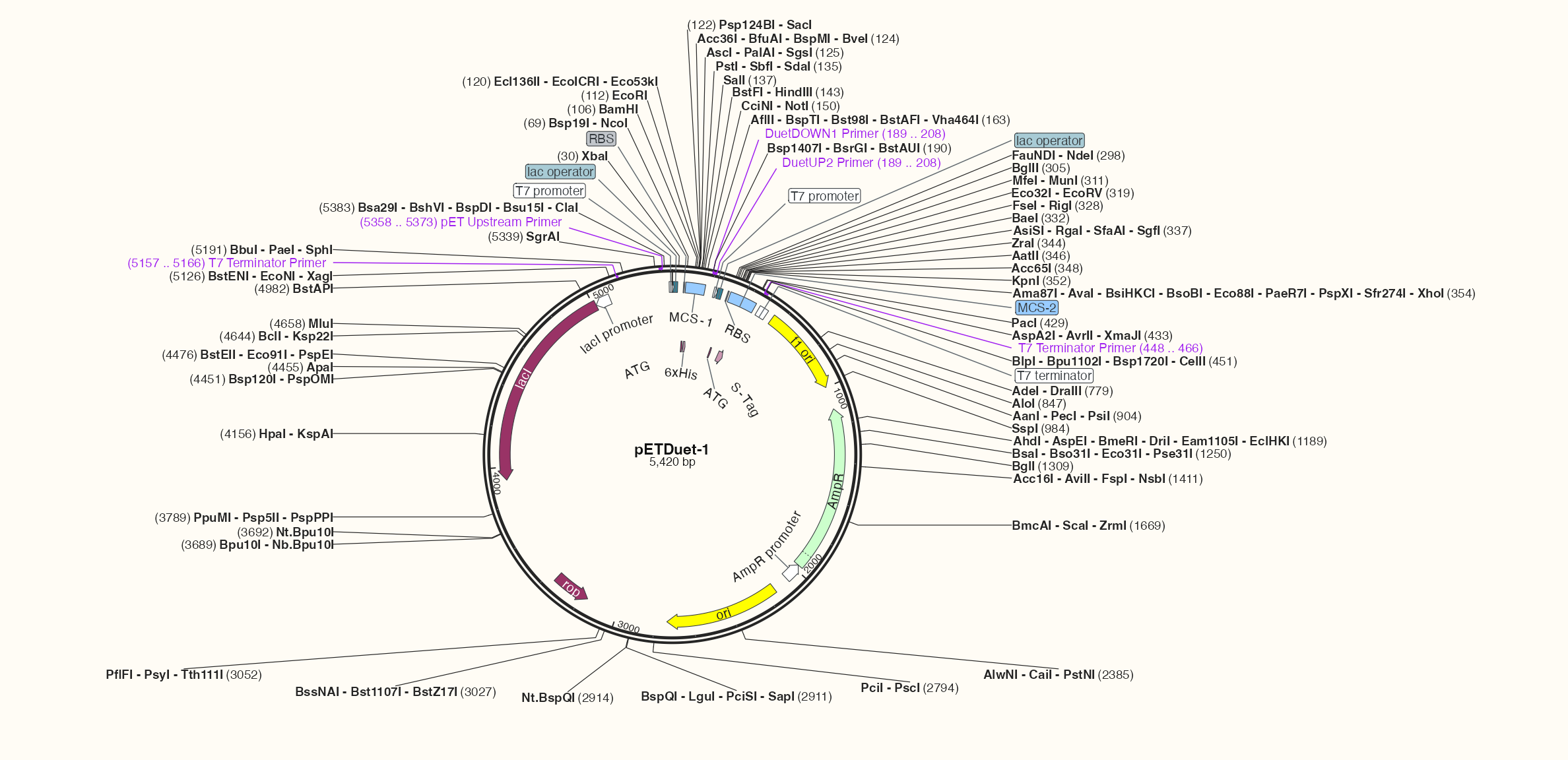

20 个特征、5 个参考引物、58 个合并切点构成输入。默认 feature 配色保留紫红编码区域、浅绿抗性基因、黄色复制起点和蓝色调控注释；引物为紫色，与本站其他图的相同语义保持一致。密集标签对尺寸敏感，下载原图或打开大图阅读。

显式视野将密集图固定在文档给出的导出尺寸。label_fit = "shrink" 允许短特征文字缩至 2.5 mm；仍放不下的文字保留为外置标签。预览和保存应使用相同的 16.5 × 8 in 尺寸。

代码ggsave("pETDuet-1-map.png", p_show_plasmid, width = 16.5, height = 8, units = "in", dpi = 144)