2.4 比较基因邻域

本页目录

本页准备
1. 提取实际 CDS 与编码 DNA
2. 显式声明成员和序列对
3. 聚焦到可比较的邻域
4. 将有证据的蛋白区间投影到两端 CDS
完成后检查
保存本页结果

比较两条质粒的 AmpR 邻域。先核对真实编码 DNA，再建立对应关系，最后聚焦到 CDS 两侧各 200 bp。

本页准备

只需随包数据，无需下载文件或重新比对。先加载包和本例的可选排版设置。

准备代码 · 在本页运行一次

代码library(ggchord)
doc_background <- "#FFFCF5"
identity_palette <- c("#303B71", "#36537D", "#269B82", "#A5D52C", "#ECEB31")
identity_values <- c(0, 0.5, 0.8, 0.9, 1)
identity_breaks <- c(0, 50, 80, 90, 100)
doc_legend_theme <- theme(
  legend.title = element_text(size = 13, face = "bold"),
  legend.text = element_text(size = 11),
  legend.key.width = unit(9, "mm"), legend.key.height = unit(5, "mm"),
  legend.spacing.x = unit(9, "mm"), legend.spacing.y = unit(7, "mm"),
  legend.margin = margin(l = 4, r = 4, unit = "mm")
)
sequence_guide <- guide_ggchord_legend(nrow = 1, theme = doc_legend_theme)
strand_guide <- guide_ggchord_legend(
  nrow = 1, override.aes = list(strand = c("+", "-")), theme = doc_legend_theme
)
identity_guide <- guide_ggchord_colourbar(
  position = "left", direction = "vertical",
  theme = theme(
    legend.key.height = unit(75, "mm"), legend.key.width = unit(5, "mm"),
    legend.title = element_text(size = 13, face = "bold"),
    legend.text = element_text(size = 11), legend.margin = margin(r = 7, unit = "mm")
  )
)
doc_theme <- theme_ggchord_publication(
  axis.text = element_text(size = 11),
  axis.text.check.overlap = TRUE
) +
  theme(
    legend.position = "bottom",
    legend.title = element_text(size = 13, face = "bold"),
    legend.text = element_text(size = 11),
    legend.key.width = unit(9, "mm"), legend.key.height = unit(5, "mm"),
    legend.spacing.x = unit(9, "mm"), legend.spacing.y = unit(7, "mm"),
    legend.box.spacing = unit(6, "mm"),
    plot.background = element_rect(fill = doc_background, colour = NA),
    panel.background = element_blank(),
    plot.title = element_text(face = "bold", size = 18),
    plot.subtitle = element_text(size = 10, colour = "#5C625A"),
    plot.margin = margin(14, 18, 14, 18)
  )
doc_axis <- function(coordinates = "relative") {
  scale_seq_position_continuous(
    coordinates = coordinates, n.breaks = 3, minor_breaks = NULL,
    labels = function(x) format(x, scientific = FALSE, big.mark = ",", trim = TRUE)
  )
}

1. 提取实际 CDS 与编码 DNA

选择随包 pUC19 与 pETDuet-1 的 AmpR 注释，保留 ID、坐标、链和文字。按负链进行反向互补，保证比较的是同一生物学方向的 DNA，而非仅比较注释名称。

代码library(dplyr)
data(plasmid_example_pUC19)
data(plasmid_example_pETDuet_1)
homolog_source <- bind_rows(plasmid_example_pUC19, plasmid_example_pETDuet_1)
homolog_seq <- homolog_source |>
  select(accver, length)
cluster_features <- homolog_source |>
  find_common_features() |>
  filter(type == "CDS", anno == "AmpR") |>
  select(accver, start, end, strand, anno) |>
  arrange(match(accver, homolog_source$accver)) |>
  mutate(feature_id = paste(accver, start, end, sep = ":"))
# Membership is computed from exact strand-corrected CDS DNA equality, not gene names.
reverse_complement <- function(sequence) {
  bases <- strsplit(sequence, "")[[1]]
  chartr("ACGT", "TGCA", paste(rev(bases), collapse = ""))
}
coding_sequences <- cluster_features |>
  left_join(select(homolog_source, accver, sequence), by = "accver") |>
  rowwise() |>
  mutate(
    coding_dna = substr(sequence, start, end),
    coding_dna = if (strand == "-") reverse_complement(coding_dna) else coding_dna
  ) |>
  ungroup()
cds_dna <- pull(coding_sequences, coding_dna)

cluster_features 应有两条实际 CDS，cds_dna 保存各自的定向编码序列。本例的严格目标是完全相同 DNA；一般同源性分析可使用外部比对与聚类结果，不能要求所有同源基因完全一致。

2. 显式声明成员和序列对

用编码 DNA 的完全一致性建立成员表；不同 DNA 不会因为都叫 AmpR 就分入同一组。

代码membership <- tibble(
  feature_id = cluster_features$feature_id,
  cluster_id = paste0("exact_CDS_", match(cds_dna, unique(cds_dna)))
)
homologs <- link_ggchord_clusters(cluster_features, membership,
  pairs = tibble(qaccver = homolog_seq$accver[1], saccver = homolog_seq$accver[2])
)
loci <- find_ggchord_loci(homolog_seq, cluster_features,
  targets = cluster_features$feature_id[cluster_features$anno == "AmpR"][1], upstream = 100, downstream = 100
)

查看 membership 与 homologs$report$comparisons、$members。连接工具消费已有分组，不计算新的序列比对。未知成员与歧义 paralog 会被报告；只有明确选择 paralogs = "all" 才请求受界限约束的所有组合。

3. 聚焦到可比较的邻域

全长质粒图会把单个 CDS 压得很小。这里从两条真实 CDS 的源范围构建窗口，两侧各增加 200 bp；原始序列表与注释表保持不变。

代码# Compare equivalent local windows instead of shrinking one gene on full plasmids.
homolog_windows <- cluster_features |>
  select(accver, start, end)
local_homologs <- focus_ggchord_data(homolog_seq, homologs$data, cluster_features,
  loci = homolog_windows, expand = 200
)
p_homologs <- ggchord(
  seq_data = local_homologs$seq_data,
  ribbon_data = local_homologs$ribbon_data, gene_data = local_homologs$gene_data
) +
  geom_link_ribbon(fill = "#269B82", alpha = .65) +
  geom_seq(colour = "#233E4A", show.legend = FALSE) +
  geom_feature(
    data = local_homologs$gene_data, feature_fill = "#F1D334",
    position = position_strand(.10), width = .07
  ) +
  geom_feature_label_repel(data = local_homologs$gene_data, size = 4, label_fit = "shrink") +
  geom_seq_label(size = 4) +
  geom_seq_break() +
  coord_collinear() +
  doc_axis("source") +
  doc_theme
p_homologs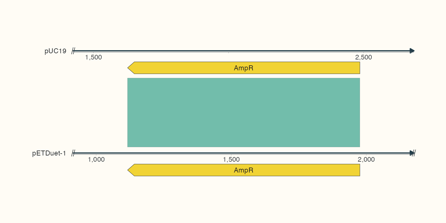

两条质粒的 AmpR 邻域：相同 CDS、200 bp 侧翼与源坐标 · 点击放大查看

两条金色箭头表示已核对的相同编码序列，紫色带连接对应 CDS 范围，内部文字直接标明 AmpR。刻度来自各自源序列，因此同一个横向位置可以显示不同源坐标。断点标记说明图中只保留了局部窗口。

local_homologs$report 记录保留与裁剪情况。窗口外的基因没有显示，不表示它们不存在。区间连接表达分组对应范围，不是逐碱基比对；跨分段注释的外包范围也不等于外显子级对应。

4. 将有证据的蛋白区间投影到两端 CDS

代码# Exact CDS DNA equality supplies evidence for these selected ungapped residues.
matching <- homologs$data |>
  slice_head(n = 1)
paired_coding <- cluster_features |>
  mutate(phase = 0)
paired_cds <- build_ggchord_cds(paired_coding)
protein_link <- tibble(
  qfeature_id = matching$qfeature_id, sfeature_id = matching$sfeature_id,
  qstart = 1, qend = 20, sstart = 1, send = 20
)
projected_links <- project_ggchord_links(protein_link, paired_cds, ungapped = TRUE)
projected_links

项目	结果
投影到基因组的注释行数	1
投影后的核苷酸连接行数	1

这里选择相同 CDS 的前 20 个残基，因此 ungapped = TRUE 有实际序列依据。普通 BLASTp HSP 不能仅凭两端跨度相等作出这个断言。工具保留源蛋白统计，不把蛋白相似度冒充核苷酸相似度。

完成后检查

两个内部标签都应为 AmpR，箭头保留真实负链方向。对应关系来自编码 DNA；源坐标与聚焦报告解释了局部显示。保存时使用 10 × 5 in 的明确尺寸。

下一步：真实 BLASTp 查询区间读取、CDS 投影及分段限制、独立局部窗口。

保存本页结果

在工作目录中保存刚刚创建的图；预览时使用相同宽高。

代码ggsave("ampR-neighbourhood.png", p_homologs, width = 10, height = 5, units = "in", dpi = 144)