全站目录 · 按任务查找
放置和调整标签
在保持注释几何的前提下安排文字:先选输出尺寸和标签子集,再选择自动或固定位置。
本页准备
在新的 R 会话中先运行下方代码,再按页面顺序继续。配色和排版是可选的显示设置,输入只选择需要的列。
准备代码 · 在本页运行一次
代码
library(ggchord)
library(dplyr)
data(seq_data_example)
data(ribbon_data_example)
data(gene_data_example)
seqs <- seq_data_example |>
  select(accver, length)
links <- ribbon_data_example |>
  select(qaccver, saccver, qstart, qend, sstart, send)
# The fixture preserves biological strands separately from its old display strands.
genes <- gene_data_example |>
  transmute(accver, start, end, strand = source_strand)

# Optional appearance choices; none of these columns or scales is required input.
library(ggchord)
seq_palette <- setNames(
  c("#E64B35", "#233E4A", "#269B82", "#D59B17"),
  c("MT108731.1", "MT118296.1", "OQ646790.1", "OR222515.1")
)
gene_palette <- c("+" = "#CE1536", "-" = "#346B9D", "." = "#8291A6")

library(ggchord)
doc_background <- "#FFFCF5"
identity_palette <- c("#303B71", "#36537D", "#269B82", "#A5D52C", "#ECEB31")
identity_values <- c(0, 0.5, 0.8, 0.9, 1)
identity_breaks <- c(0, 50, 80, 90, 100)
doc_legend_theme <- theme(
  legend.title = element_text(size = 13, face = "bold"),
  legend.text = element_text(size = 11),
  legend.key.width = unit(9, "mm"), legend.key.height = unit(5, "mm"),
  legend.spacing.x = unit(9, "mm"), legend.spacing.y = unit(7, "mm"),
  legend.margin = margin(l = 4, r = 4, unit = "mm")
)
sequence_guide <- guide_ggchord_legend(nrow = 1, theme = doc_legend_theme)
strand_guide <- guide_ggchord_legend(
  nrow = 1, override.aes = list(strand = c("+", "-")), theme = doc_legend_theme
)
identity_guide <- guide_ggchord_colourbar(
  position = "left", direction = "vertical",
  theme = theme(
    legend.key.height = unit(75, "mm"), legend.key.width = unit(5, "mm"),
    legend.title = element_text(size = 13, face = "bold"),
    legend.text = element_text(size = 11), legend.margin = margin(r = 7, unit = "mm")
  )
)
doc_theme <- theme_ggchord_publication(
  axis.text = element_text(size = 11),
  axis.text.check.overlap = TRUE
) +
  theme(
    legend.position = "bottom",
    legend.title = element_text(size = 13, face = "bold"),
    legend.text = element_text(size = 11),
    legend.key.width = unit(9, "mm"), legend.key.height = unit(5, "mm"),
    legend.spacing.x = unit(9, "mm"), legend.spacing.y = unit(7, "mm"),
    legend.box.spacing = unit(6, "mm"),
    plot.background = element_rect(fill = doc_background, colour = NA),
    panel.background = element_blank(),
    plot.title = element_text(face = "bold", size = 18),
    plot.subtitle = element_text(size = 10, colour = "#5C625A"),
    plot.margin = margin(14, 18, 14, 18)
  )
doc_axis <- function(coordinates = "relative") {
  scale_seq_position_continuous(
    coordinates = coordinates, n.breaks = 3, minor_breaks = NULL,
    labels = function(x) format(x, scientific = FALSE, big.mark = ",", trim = TRUE)
  )
}
选择布局
基因标签提供 "auto"、"radial"、"arc" 布局。通用注释标签还支持优先 内部放置的默认 "feature" 和外部 "callout"。应按实际图层选择已记录的取值, 这些布局并不是可在所有入口互换的预设。
代码
label_data <- gene_data_example |>
  filter(anno != "hypothetical protein") |>
  transmute(accver, start, end, strand = source_strand, anno)
p_labels <- ggchord(seq_data = seqs, gene_data = genes) +
  geom_seq() +
  geom_gene() +
  geom_gene_label_repel(data = label_data, label_layout = "auto", size = 4, label_wrap = 22) +
  geom_seq_label(size = 4) +
  coord_collinear() +
  doc_axis() +
  scale_seq_colour_manual(values = seq_palette) +
  scale_gene_fill_manual(values = gene_palette) +
  doc_theme
p_labels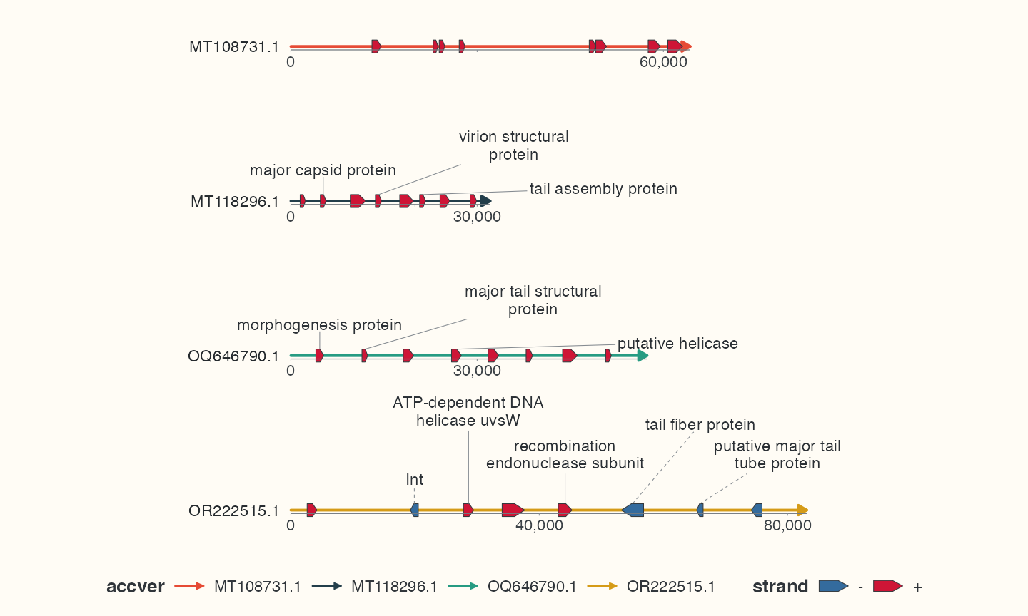
固定与自动放置
手动 label_rotation、径向/周向位移和方向控制使用 geom_gene_label() 或 geom_feature_label()。自动层拒绝这些手动控制,应选择 label_layout 或删除手动参数。 固定文字样式使用受支持的 size、colour、family。
在支持的入口中,label_fit、label_wrap、label_max_lines、label_min_size 控制适配。缩小字号须显式选择且有下限。无法放置的标签可能移位或隐藏,注释 几何仍保留。应在最终导出尺寸查看 label_fit_diagnostics、label_diagnostics。
跨层匹配锚点
共线性模式中,省略的注释标签 Position 可继承无歧义的匹配注释层。 唯一 feature_id 允许重排或取子集,但标识、区间、链仍须一致。 多个匹配层需要明确 Position 或无歧义 ID。先选最终设备尺寸再预览;调整 Plots 面板会改变可用空间。
对照三种基因标签布局
代码
# Compare layouts with at most the first and last informative label per sequence.
comparison_labels <- label_data |>
  group_by(accver) |>
  filter(row_number() %in% c(1L, n())) |>
  ungroup()
label_plots <- lapply(c("auto", "radial", "arc"), function(layout) {
  ggchord(seq_data = seqs, gene_data = genes) +
    geom_seq() +
    geom_gene() +
    geom_gene_label_repel(data = comparison_labels, label_layout = layout, size = 4, label_wrap = 22) +
    geom_seq_label(size = 4) +
    scale_seq_colour_manual(values = seq_palette, name = "Sequence",
      guide = guide_ggchord_legend(nrow = 2, theme = doc_legend_theme)) +
    scale_gene_fill_manual(values = gene_palette, breaks = c("+", "-"), name = "Strand", guide = strand_guide) +
    coord_chord(xlim = c(-1.8, 1.8), ylim = c(-1.6, 1.6)) +
    theme_ggchord_publication(axis = element_blank()) +
    doc_legend_theme +
    theme(
      legend.position = "bottom",
      plot.background = element_rect(fill = doc_background, colour = NA),
      panel.background = element_blank()
    ) +
    labs(title = layout)
})
names(label_plots) <- c("auto", "radial", "arc")
p_manual_labels <- ggchord(seq_data = seqs, gene_data = genes) +
  geom_seq() +
  geom_gene() +
  geom_gene_label(data = label_data, label_rotation = 30) +
  coord_collinear()
label_plots$auto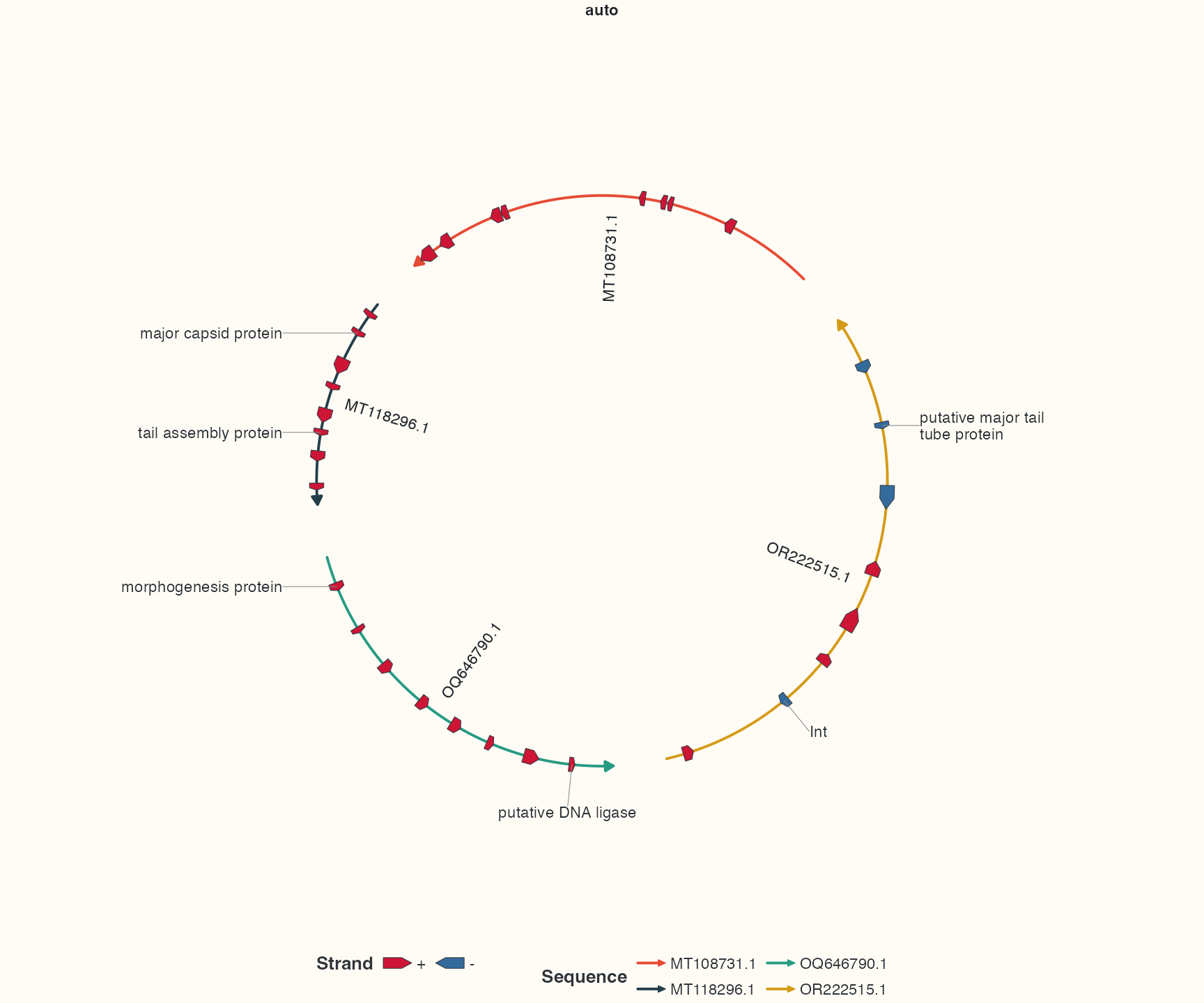
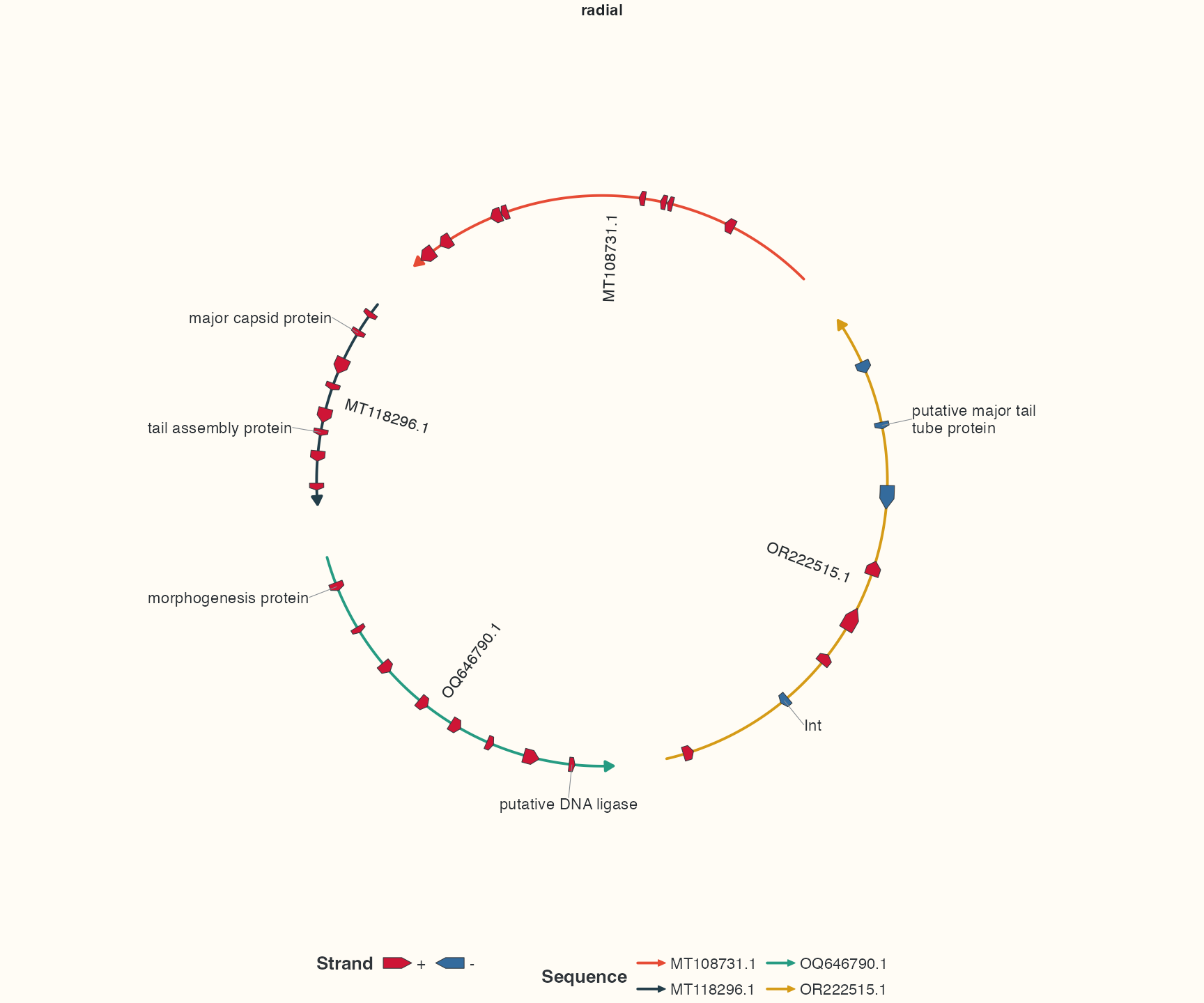
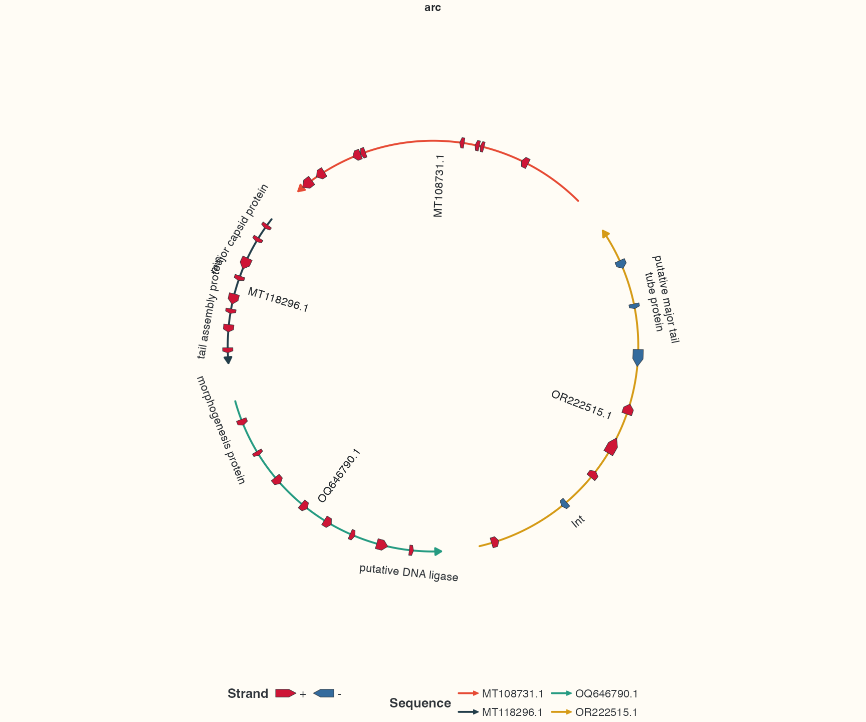
每条序列最多选最前和最后两个有信息的标签,保留全部基因箭头,便于比较文字方向。 打印 label_plots$auto、$radial 或 $arc 查看候选图。三图输入和请求字号相同, 仅布局选择不同。auto 在适用处使用共享侧列,radial 跟随局部轮廓,arc 跟随序列切线。 p_manual_labels 展示独立固定标签入口,显式旋转不属于自动 repel 图层。 通用注释标签还可选内部优先/callout,密集混合注释见完整圆图, 继承或显式 Position 锚点见堆叠。
完成后检查
三张布局对照使用同一输入。判断可读性时同时看文字方向、连线和隐藏原因;没有标签不等于注释丢失。