0.16.6 文档
全站目录 · 按任务查找
2.5 局部、锚定与分段
为已有输入选择局部窗口或分段视图,同时保留原始位置与显示变换的区别。
本页准备
在新的 R 会话中先运行下方代码,再按页面顺序继续。配色和排版是可选的显示设置,输入只选择需要的列。
准备代码 · 在本页运行一次
代码
library(ggchord)
library(dplyr)
data(seq_data_example)
data(ribbon_data_example)
data(gene_data_example)
seqs <- seq_data_example |>
  select(accver, length)
links <- ribbon_data_example |>
  select(qaccver, saccver, qstart, qend, sstart, send)
# The fixture preserves biological strands separately from its old display strands.
genes <- gene_data_example |>
  transmute(accver, start, end, strand = source_strand)

# Optional appearance choices; none of these columns or scales is required input.
library(ggchord)
seq_palette <- setNames(
  c("#E64B35", "#233E4A", "#269B82", "#D59B17"),
  c("MT108731.1", "MT118296.1", "OQ646790.1", "OR222515.1")
)
gene_palette <- c("+" = "#CE1536", "-" = "#346B9D", "." = "#8291A6")

library(ggchord)
doc_background <- "#FFFCF5"
identity_palette <- c("#303B71", "#36537D", "#269B82", "#A5D52C", "#ECEB31")
identity_values <- c(0, 0.5, 0.8, 0.9, 1)
identity_breaks <- c(0, 50, 80, 90, 100)
doc_legend_theme <- theme(
  legend.title = element_text(size = 13, face = "bold"),
  legend.text = element_text(size = 11),
  legend.key.width = unit(9, "mm"), legend.key.height = unit(5, "mm"),
  legend.spacing.x = unit(9, "mm"), legend.spacing.y = unit(7, "mm"),
  legend.margin = margin(l = 4, r = 4, unit = "mm")
)
sequence_guide <- guide_ggchord_legend(nrow = 1, theme = doc_legend_theme)
strand_guide <- guide_ggchord_legend(
  nrow = 1, override.aes = list(strand = c("+", "-")), theme = doc_legend_theme
)
identity_guide <- guide_ggchord_colourbar(
  position = "left", direction = "vertical",
  theme = theme(
    legend.key.height = unit(75, "mm"), legend.key.width = unit(5, "mm"),
    legend.title = element_text(size = 13, face = "bold"),
    legend.text = element_text(size = 11), legend.margin = margin(r = 7, unit = "mm")
  )
)
doc_theme <- theme_ggchord_publication(
  axis.text = element_text(size = 11),
  axis.text.check.overlap = TRUE
) +
  theme(
    legend.position = "bottom",
    legend.title = element_text(size = 13, face = "bold"),
    legend.text = element_text(size = 11),
    legend.key.width = unit(9, "mm"), legend.key.height = unit(5, "mm"),
    legend.spacing.x = unit(9, "mm"), legend.spacing.y = unit(7, "mm"),
    legend.box.spacing = unit(6, "mm"),
    plot.background = element_rect(fill = doc_background, colour = NA),
    panel.background = element_blank(),
    plot.title = element_text(face = "bold", size = 18),
    plot.subtitle = element_text(size = 10, colour = "#5C625A"),
    plot.margin = margin(14, 18, 14, 18)
  )
doc_axis <- function(coordinates = "relative") {
  scale_seq_position_continuous(
    coordinates = coordinates, n.breaks = 3, minor_breaks = NULL,
    labels = function(x) format(x, scientific = FALSE, big.mark = ",", trim = TRUE)
  )
}
保留来源的局部聚焦
代码
focus_loci <- tibble(
  accver = seqs$accver,
  start = floor(seqs$length * .25), end = floor(seqs$length * .75)
)
focused <- focus_ggchord_data(seqs, links, genes, loci = focus_loci)
p_focus <- ggchord(
  seq_data = focused$seq_data, ribbon_data = focused$ribbon_data,
  gene_data = focused$gene_data
) +
  geom_seq() +
  geom_link_ribbon(fill = "#6BAFA6", alpha = .5) +
  geom_gene() +
  geom_seq_break() +
  geom_seq_label(size = 4) +
  scale_seq_colour_manual(values = seq_palette) +
  scale_gene_fill_manual(values = gene_palette) +
  doc_axis("source") +
  coord_collinear() +
  doc_theme
p_focus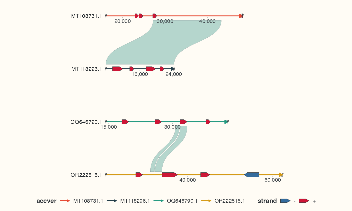
focus 把保留位置移到局部一基坐标,同时保留源原点、截断标记与报告。 boundary = "trim" 可按线性显示投影裁剪连接,不重新比对序列;缩放后的比对长度 带估计标记。coordinates = "source" 恢复源坐标轴标签,重复聚焦后同样适用。
独立窗口与局部翻转
代码
windows <- tibble(
  accver = rep(seqs$accver[1], 2),
  start = c(1, floor(seqs$length[1] * .65)), end = c(floor(seqs$length[1] * .4), seqs$length[1]),
  locus_id = c("left_window", "right_window"), row_id = seqs$accver[1], orientation = c(1, -1)
)
segmented <- segment_ggchord_data(slice_head(seqs, n = 1), windows = windows)
p_segments <- ggchord(seq_data = segmented$seq_data) +
  geom_seq() +
  coord_collinear(segments = segmented$segments, segment_gap = 2000)
p_segments各窗口有可逆的源映射,被省略的间隙没有映射。map_ggchord_position() 把显式源 位置映射到图中,供普通 ggplot2 注释使用。多个窗口共享源序列时应指定窗口 ID。 显示方向不表示原始链发生改变。
显式生物学关系
find_ggchord_loci() 按声明的注释/名称查询选择位置。 link_ggchord_clusters() 要求显式成员表和序列对,基因名称相同不构成同源证据。 filter_ggchord_ribbons()、deduplicate_ggchord_ribbons()、 merge_ggchord_ribbons() 整理已有比对,保留源成员和估计长度标记。 聚束和密度统计汇总已提供连接,不创建新的序列比对。
按源坐标放置普通注释
代码
source_position <- focus_loci$start[1] + 100
source_mark <- map_ggchord_position(p_focus, seqs$accver[1], source_position, source = TRUE)
p_marked <- p_focus +
  ggplot2::geom_point(
    data = source_mark, aes(x, y),
    inherit.aes = FALSE, colour = "#D59B17", size = 3
  )
p_marked先运行focus 例子。辅助函数返回第一个所选窗口起点后 100 bp 位置的笛卡尔 x/y, 不把全部普通 ggplot2 坐标变成基因组 bp。分段视图应选窗口 ID,检查落在省略间隙 的位置,不跨间隙外推。区域 选择来自明确注释/同源分组 证据时见显式同源关系。
完成后检查
关注裁剪报告、断点与源坐标。被省略的间隙没有映射;显示翻转不应直接解释为生物学倒位。