0.16.6 documentation

Site guide · find your task

Setup and learning paths

HomeInstall and prepare the environmentChoose your learning module

Module I · Chord

1.1 Tables and field meanings1.2 Produce and import comparisons1.3 Build the layers step by step1.4 Direction, curvature and clearance1.5 Filter and summarize links1.6 Full source-file workflow1.7 Complete chord showcase

Module II · Collinear

2.1 Reuse chord input tables2.2 Switch coordinates and add layers2.3 Routes, clearance and the ruler2.4 Compare CDS neighbourhoods2.5 Focus, anchors and segments2.6 Complete collinear showcase

Module III · Plasmid

3.1 DNA, annotations and 13 references3.2 From a circle to annotation layers3.3 Features, primers and restriction3.4 Thirteen plasmid references3.5 Complete plasmid cases

Consult as needed · Data and layers

Prepare tables and coordinatesImport and convert dataImport nucleotide and protein alignmentsProject protein intervals to genomic coordinatesFeatures, stacking and genomic decorationLabels and local placementQuantitative tracksMappings, scales, guides and themesSet values by sequence and strandCommon adjustments and grammarExport, preview and diagnostics

Learning map and reference

Articles and complete workflowsFunction referenceReproducible galleryFrequently asked questionsMigrate to the candidate APITerminology and design sourcesDevelopment status and changes

3.5 Complete plasmid cases

On this page

• Prepare this page
• Use a source-backed sequence
• Compose independent layers
• Read the annotation layers
• Choose the displayed sites deliberately
• Understand catalogue and label limits
• Adapt the workflow
• Check your result
• Save this result
• Complete example: a dense pETDuet-1 map

Build a readable plasmid map from bundled pUC19 DNA, with separate annotation, primer and restriction layers. Keep display choices separate from complete results.

Prepare this page

In a fresh R session, run the code below, then follow this page in order. Colours and layout are optional display choices; inputs select only the fields needed.

Preparation code — run once on this page

Code

library(ggchord)
feature_palette <- c(
  CDS = "#993366", promoter = "#31849B", rep_origin = "#F1E51D",
  primer_bind = "#A020F0", misc_feature = "#A6ACB3", protein_bind = "#31849B"
)

library(ggchord)
doc_background <- "#FFFCF5"
identity_palette <- c("#303B71", "#36537D", "#269B82", "#A5D52C", "#ECEB31")
identity_values <- c(0, 0.5, 0.8, 0.9, 1)
identity_breaks <- c(0, 50, 80, 90, 100)
doc_legend_theme <- theme(
  legend.title = element_text(size = 13, face = "bold"),
  legend.text = element_text(size = 11),
  legend.key.width = unit(9, "mm"), legend.key.height = unit(5, "mm"),
  legend.spacing.x = unit(9, "mm"), legend.spacing.y = unit(7, "mm"),
  legend.margin = margin(l = 4, r = 4, unit = "mm")
)
sequence_guide <- guide_ggchord_legend(nrow = 1, theme = doc_legend_theme)
strand_guide <- guide_ggchord_legend(
  nrow = 1, override.aes = list(strand = c("+", "-")), theme = doc_legend_theme
)
identity_guide <- guide_ggchord_colourbar(
  position = "left", direction = "vertical",
  theme = theme(
    legend.key.height = unit(75, "mm"), legend.key.width = unit(5, "mm"),
    legend.title = element_text(size = 13, face = "bold"),
    legend.text = element_text(size = 11), legend.margin = margin(r = 7, unit = "mm")
  )
)
doc_theme <- theme_ggchord_publication(
  axis.text = element_text(size = 11),
  axis.text.check.overlap = TRUE
) +
  theme(
    legend.position = "bottom",
    legend.title = element_text(size = 13, face = "bold"),
    legend.text = element_text(size = 11),
    legend.key.width = unit(9, "mm"), legend.key.height = unit(5, "mm"),
    legend.spacing.x = unit(9, "mm"), legend.spacing.y = unit(7, "mm"),
    legend.box.spacing = unit(6, "mm"),
    plot.background = element_rect(fill = doc_background, colour = NA),
    panel.background = element_blank(),
    plot.title = element_text(face = "bold", size = 18),
    plot.subtitle = element_text(size = 10, colour = "#5C625A"),
    plot.margin = margin(14, 18, 14, 18)
  )
doc_axis <- function(coordinates = "relative") {
  scale_seq_position_continuous(
    coordinates = coordinates, n.breaks = 3, minor_breaks = NULL,
    labels = function(x) format(x, scientific = FALSE, big.mark = ",", trim = TRUE)
  )
}

The preparation above declares the palette and shared appearance.

Use a source-backed sequence

The bundled plasmid_example_pUC19 is copied from the repository’s original examples/plasmid/pUC19.fna; bases and sequence identity are not edited for display. The workflow uses the package’s source-backed recognition catalogues. It needs no network request or experimental measurements fabricated for the figure.

Code

library(dplyr)
data(plasmid_example_pUC19)
plasmid_seq <- plasmid_example_pUC19 |>
  select(accver, length)
plasmid_feature_source <- find_common_features(plasmid_example_pUC19)
# Dedicated primer layers already show bindings; avoid duplicate primer annotations.
plasmid_features <- plasmid_feature_source |>
  filter(type != "primer_bind") |>
  select(accver, start, end, strand, type, anno)
plasmid_primers <- find_primer_bindings(plasmid_example_pUC19, set = "universal")
plasmid_sites <- find_restriction_sites(plasmid_example_pUC19)
display_sites <- filter_restriction_sites(plasmid_sites, enzymes = c("EcoRI", "BamHI", "HindIII"))
primer_names <- primer_catalog(set = "universal")

Inspect plasmid_features, plasmid_primers and display_sites to distinguish complete search results from display choices.

Compose independent layers

Add the backbone, annotations, labels, primers and restriction sites in that order. Features and their labels share one Position; each layer reads its own data.

Code

plasmid_position <- position_feature_stack(spacing = .10, base_position = position_plasmid())
p_plasmid <- ggchord(seq_data = plasmid_seq) +
  geom_seq(seq_style = "double") +
  geom_feature_plasmid(aes(feature_fill = type), data = plasmid_features, position = plasmid_position) +
  geom_feature_label_repel(
    data = plasmid_features, position = plasmid_position,
    size = 4
  ) +
  geom_primer(data = plasmid_primers, colour = "#A020F0") +
  geom_primer_label_repel(data = plasmid_primers, colour = "#A020F0", max_overlaps = 0, size = 3) +
  geom_restriction_site(data = display_sites, colour = "#29364B", label_size = 3, leader = "radial") +
  geom_seq_center_label() +
  scale_feature_fill_manual(values = feature_palette) +
  scale_seq_position_continuous() +
  coord_circular(rotation = 90) +
  theme_ggchord_plasmid() +
  theme(
    legend.title = element_text(size = 13, face = "bold"),
    legend.text = element_text(size = 11),
    legend.spacing.x = unit(9, "mm"), legend.spacing.y = unit(7, "mm"),
    plot.background = element_rect(fill = doc_background, colour = NA),
    panel.background = element_blank()
  )
p_plasmid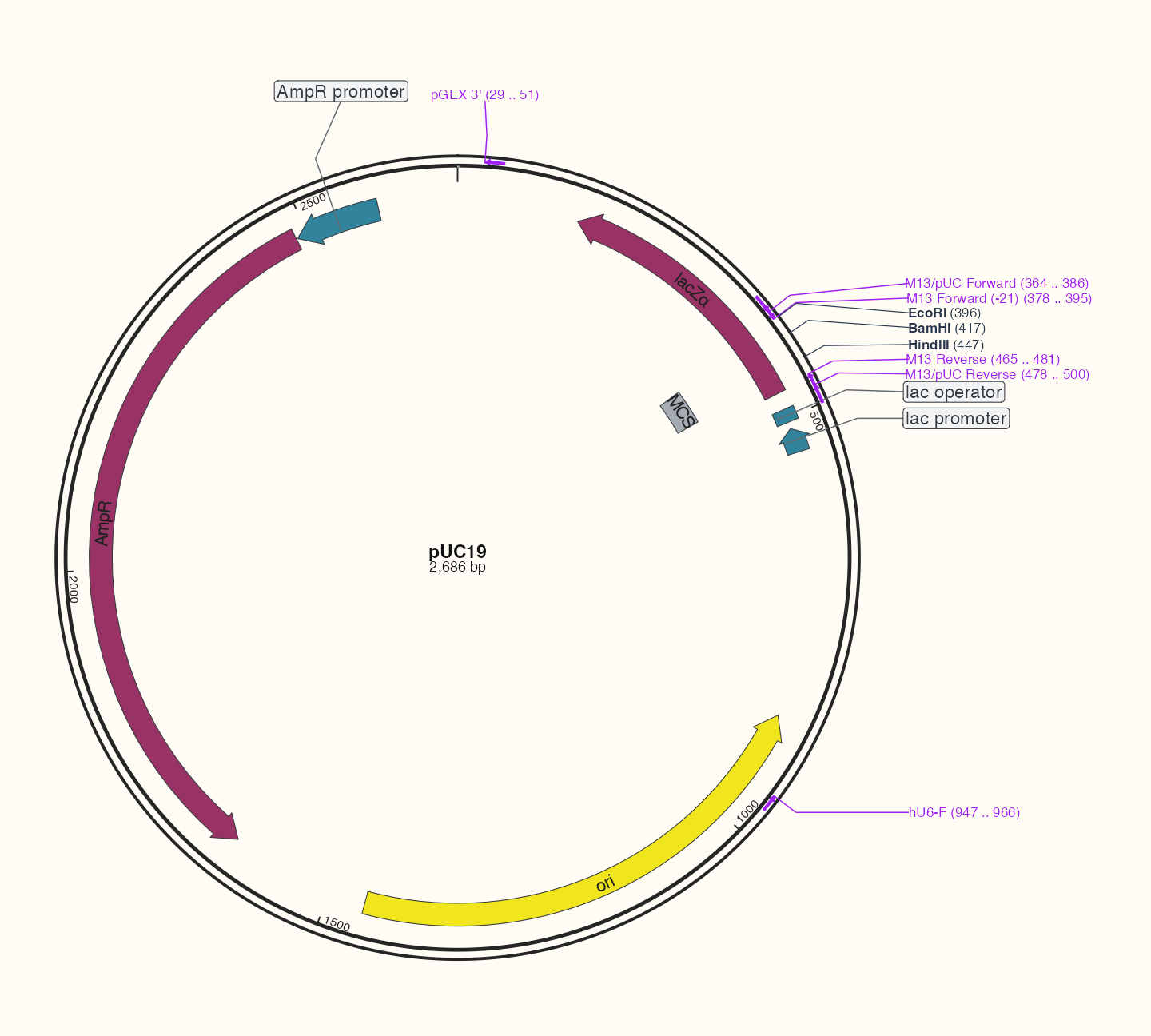

pUC19 features, exact primer hits and three selected restriction sites · Click to enlarge

Metric	Observed output
Full sequence length (bp)	2686
Annotation rows	7
Exact primer hit records	6
Enzyme match records (not distinct positions)	49845
Restriction records selected for display	3

Mixed exterior annotations share root-ordered placement, including sparse restriction labels beside primers. This example uses the dedicated plasmid theme and default feature fitting: internal text is tried before adjacent/external placement. Inspect at the final export dimensions instead of hiding crossings by shrinking text or forcing offsets.

The original annotation table is retained in plasmid_feature_source. Dedicated primer layers replace duplicate primer_bind annotations in the displayed feature table; only geometry, type and annotation text are passed to feature layers.

Read the annotation layers

The double backbone establishes one circular sequence. General features use a plasmid preset and explicit stacking Position; labels use the same Position. Primer arcs indicate binding ranges, restriction ticks indicate cleavage/display positions, and the centre label identifies the sequence and length. A cropped or filtered display does not change the full-sequence restriction count.

Choose the displayed sites deliberately

find_restriction_sites() returns all matches. This figure explicitly selects EcoRI, BamHI and HindIII so that a compact restriction cluster remains readable; plasmid_sites retains the complete search result. The reference filter uses a saved reference display set only when the complete supplied sequence matches that reference. Other tasks can select unique, six_plus or explicit enzyme names. Inspect display_sites and the site’s methylation/source columns before drawing. The reference set is a presentation choice, not a claim about an unknown sample.

Understand catalogue and label limits

primer_names exposes catalogue entries. This example searches the universal catalogue exactly; reference primer annotations and exact oligonucleotide searches have distinct provenance. Near-exact protein feature recognition has the limitations in recognition; it does not validate biological function or a primer experiment. Text can move, shrink within its explicit minimum, or hide. Keep the geometry and inspect exported label reasons at the final size rather than assuming every annotation must have text.

Adapt the workflow

For your own named DNA sequence, replace the input and inspect search results before adding geoms. For externally curated annotations, pass your feature table instead of running recognition. Use stacking and shapes for geometry, labels for fitting, and output for devices.

geom_primer_label_repel(side = "inside") keeps callouts inside the backbone, even alongside exterior restriction and feature labels. This is corrected in the 0.16.6 release; v0.16.5 can move those requested inside labels outside. The default outside placement and existing source coordinates are unchanged.

Inside restriction labels also retain their inner geometry and now report the inner side in the exported annotation registry; earlier versions mislabelled those diagnostic rows as exterior resources.

The full inside scene can still place long primer text over other feature regions. The default max_overlaps = Inf does not certify zero overlap across feature layers. Prefer the default outside field when space is tight, or use show_location = FALSE to shorten the display; inspect the result at its final size.

Check your result

Start with the centre name and length, then read positions, category colours, arrow directions and outer labels. Check enzyme names in display_sites; selecting a display subset leaves plasmid_sites intact.

Continue: Labels and local placement →

Save this result

Save the plot just created to the working directory; use matching dimensions for preview.

Code

ggsave("pUC19-map.png", p_plasmid, width = 10, height = 9, units = "in", dpi = 144)

Complete example: a dense pETDuet-1 map

Use the pUC19 example above to learn the layers, then move to the richer pETDuet-1 map. Inputs come from the bundled sequence, feature and reference-primer catalogues. The restriction subset retains unique six-base-or-longer recognition sites from commercial_all; it is not every cut made by every enzyme.

Code

library(ggchord)
library(dplyr)
data(plasmid_example_pETDuet_1)
show_plasmid <- plasmid_example_pETDuet_1 |>
  select(accver, length)
show_plasmid_features <- find_common_features(plasmid_example_pETDuet_1)
show_plasmid_primers <- find_primer_bindings(plasmid_example_pETDuet_1, set = "reference")
show_plasmid_all_sites <- find_restriction_sites(plasmid_example_pETDuet_1)
show_plasmid_sites <- filter_restriction_sites(
  show_plasmid_all_sites,
  set = "unique_6plus", parent_set = "commercial_all"
)

Code

show_plasmid_position <- position_feature_stack(
  spacing = 0.085, base_position = position_plasmid()
)
p_show_plasmid <- ggchord(show_plasmid, validate = "none") +
  geom_seq(seq_style = "double", colour = "#252525") +
  geom_feature_plasmid(data = show_plasmid_features, position = show_plasmid_position) +
  geom_feature_label_repel(
    data = show_plasmid_features, position = show_plasmid_position,
    external = TRUE, max_overlaps = 0,
    label_fit = "shrink", label_min_size = 2.5
  ) +
  geom_primer(data = show_plasmid_primers, colour = "#A020F0") +
  geom_primer_label_repel(
    data = show_plasmid_primers, colour = "#A020F0", max_overlaps = 0
  ) +
  geom_restriction_site(data = show_plasmid_sites, colour = "#252525") +
  geom_seq_center_label() +
  coord_circular(
    rotation = 90, fit = "manual",
    xlim = c(-3.4, 4.6), ylim = c(-1.6, 2.4)
  ) +
  theme_ggchord_plasmid() +
  theme(
    legend.title = element_text(size = 13, face = "bold"),
    legend.text = element_text(size = 11),
    legend.spacing.x = unit(9, "mm"), legend.spacing.y = unit(7, "mm"),
    plot.background = element_rect(fill = doc_background, colour = NA),
    panel.background = element_blank()
  )
p_show_plasmid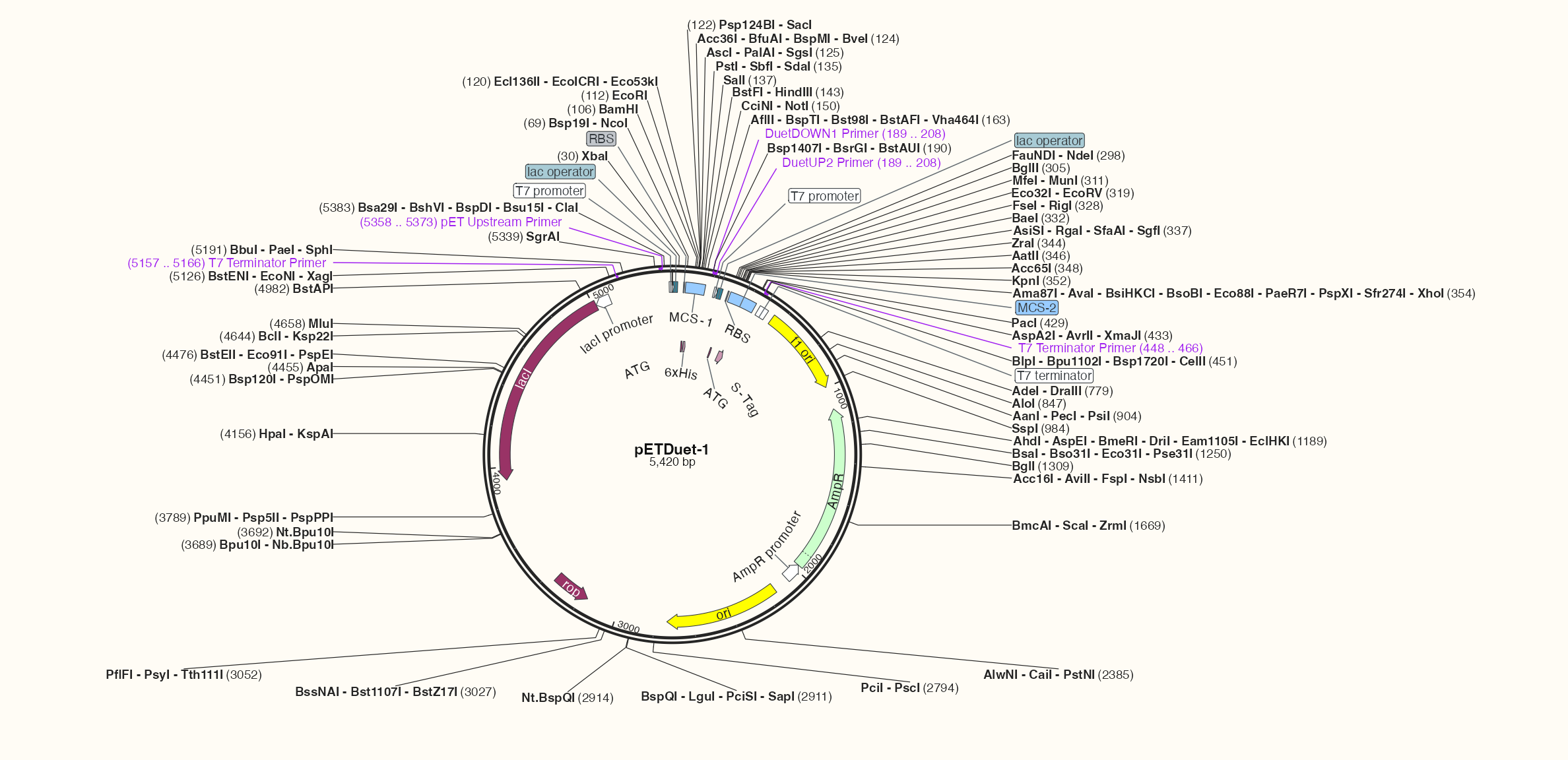

Dense pETDuet-1 map: features, reference primers and grouped restriction sites · Click to enlarge

Inputs contain 20 features, five reference primers and 58 grouped cut positions. The feature preset retains plum coding regions, mint resistance genes, yellow origins and blue regulatory features; primers are purple, consistently across this site. Dense labels depend on export size; open the full image to read them.

The explicit viewport keeps the dense map at the documented export size. label_fit = "shrink" allows short-feature labels to fit down to 2.5 mm; labels that do not fit remain callouts. Preview and save at the same 16.5 × 8 in size.

Code

ggsave("pETDuet-1-map.png", p_show_plasmid, width = 16.5, height = 8, units = "in", dpi = 144)