0.16.6 文档
全站目录 · 按任务查找
3.4 13个质粒参考案例
本页目录
- 一次准备全部案例
- 输入与识别结果
- pSB1C3:小载体与基本骨架
- pUC19:常见注释与复制起点
- pBR322:多个抗性区与方向
- pBluescript II SK(+):局部调控与短特征
- pET-28a(+):表达区与标签
- pETDuet-1:双表达单元,进入密集案例
- pDONR221:重组相关结构
- pcDNA3.1(+):表达载体的注释层级
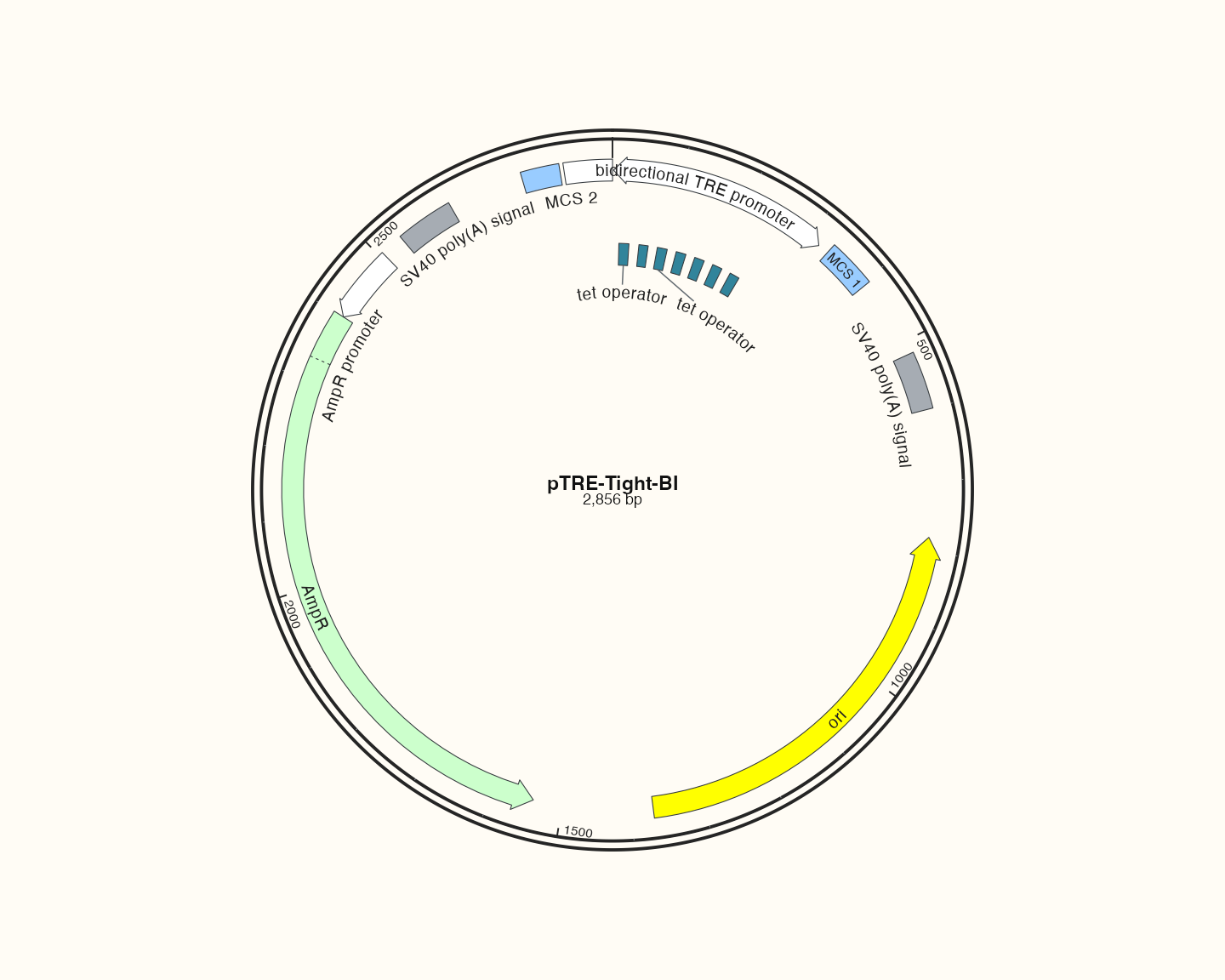
- pTRE-Tight-BI:双向调控布局
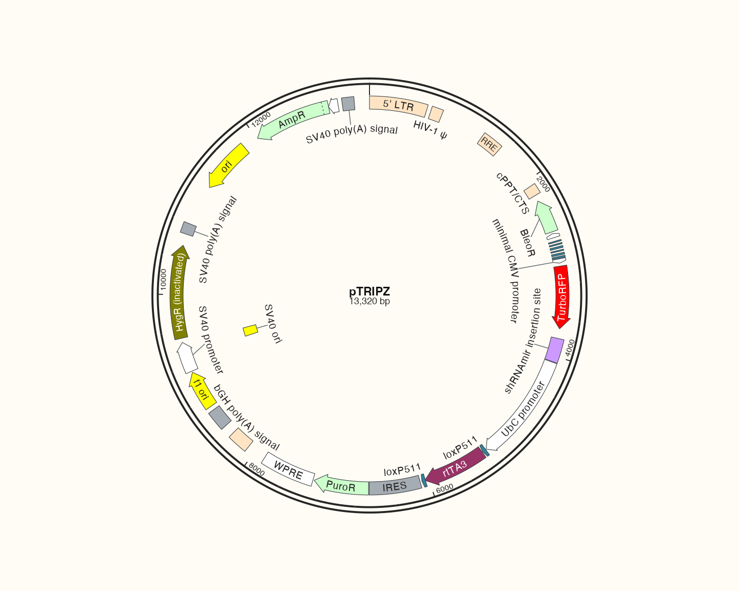
- pTRIPZ:更长序列的显示密度
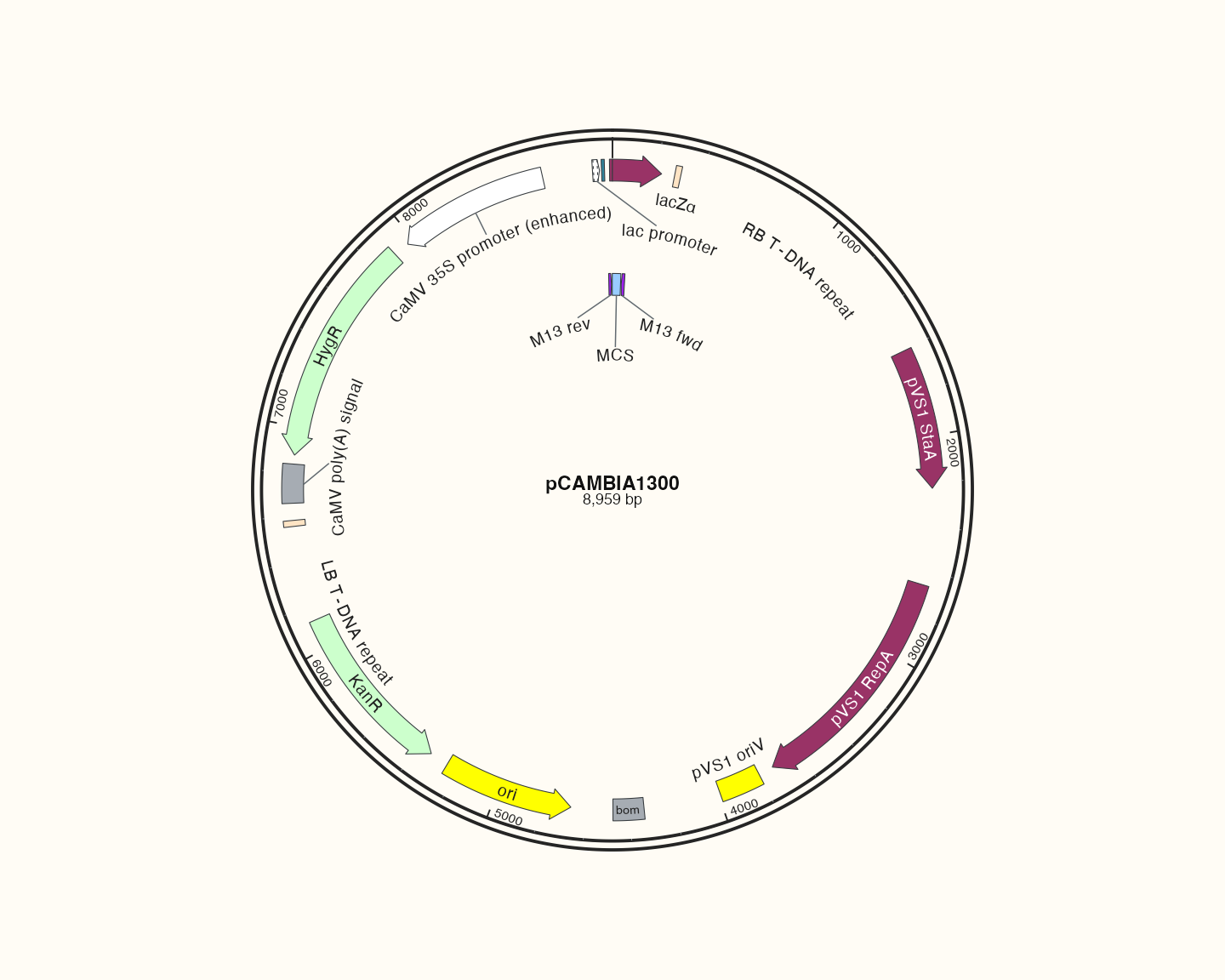
- pCAMBIA1300:较大植物载体的结构
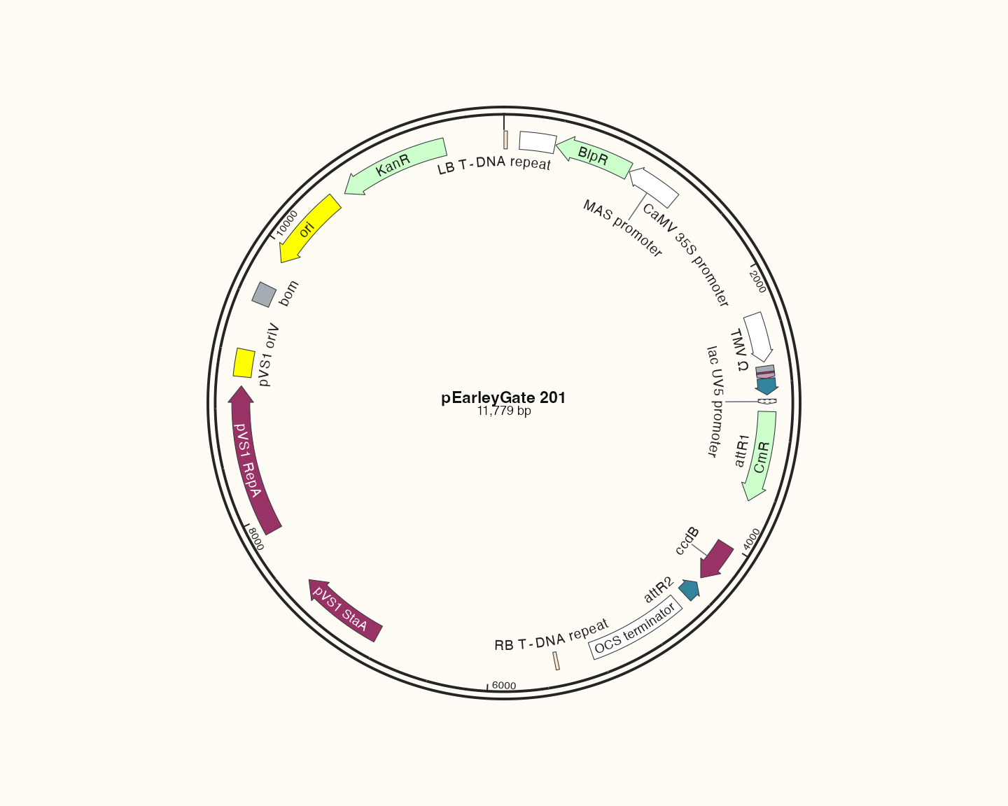
- pEarleyGate 201:另一植物载体的类别对照
- pSpCas9(BB)-2A-GFP (PX458):大型表达载体与文字适配
- 下一步
本图库包含13个独立的仓库FASTA参考记录,全部由当前代码重绘。旧版PNG和.dna文件不是本轮输出;下方只将载体用途作为学习线索,不由图形证明实验功能。完整来源和长度由随包数据及生成规则保留。
一次准备全部案例
准备代码 · 在本页运行一次
代码
library(ggchord)
doc_background <- "#FFFCF5"
identity_palette <- c("#303B71", "#36537D", "#269B82", "#A5D52C", "#ECEB31")
identity_values <- c(0, 0.5, 0.8, 0.9, 1)
identity_breaks <- c(0, 50, 80, 90, 100)
doc_legend_theme <- theme(
  legend.title = element_text(size = 13, face = "bold"),
  legend.text = element_text(size = 11),
  legend.key.width = unit(9, "mm"), legend.key.height = unit(5, "mm"),
  legend.spacing.x = unit(9, "mm"), legend.spacing.y = unit(7, "mm"),
  legend.margin = margin(l = 4, r = 4, unit = "mm")
)
sequence_guide <- guide_ggchord_legend(nrow = 1, theme = doc_legend_theme)
strand_guide <- guide_ggchord_legend(
  nrow = 1, override.aes = list(strand = c("+", "-")), theme = doc_legend_theme
)
identity_guide <- guide_ggchord_colourbar(
  position = "left", direction = "vertical",
  theme = theme(
    legend.key.height = unit(75, "mm"), legend.key.width = unit(5, "mm"),
    legend.title = element_text(size = 13, face = "bold"),
    legend.text = element_text(size = 11), legend.margin = margin(r = 7, unit = "mm")
  )
)
doc_theme <- theme_ggchord_publication(
  axis.text = element_text(size = 11),
  axis.text.check.overlap = TRUE
) +
  theme(
    legend.position = "bottom",
    legend.title = element_text(size = 13, face = "bold"),
    legend.text = element_text(size = 11),
    legend.key.width = unit(9, "mm"), legend.key.height = unit(5, "mm"),
    legend.spacing.x = unit(9, "mm"), legend.spacing.y = unit(7, "mm"),
    legend.box.spacing = unit(6, "mm"),
    plot.background = element_rect(fill = doc_background, colour = NA),
    panel.background = element_blank(),
    plot.title = element_text(face = "bold", size = 18),
    plot.subtitle = element_text(size = 10, colour = "#5C625A"),
    plot.margin = margin(14, 18, 14, 18)
  )
doc_axis <- function(coordinates = "relative") {
  scale_seq_position_continuous(
    coordinates = coordinates, n.breaks = 3, minor_breaks = NULL,
    labels = function(x) format(x, scientific = FALSE, big.mark = ",", trim = TRUE)
  )
}
代码
library(ggchord)
library(dplyr)
library(purrr)
# Thirteen unique records; the compatibility spelling pUC19c is not an extra plasmid.
catalog_objects <- c(
  "plasmid_example_pSB1C3", "plasmid_example_pUC19", "plasmid_example_pBR322",
  "plasmid_example_pBluescript_II_SK_plus", "plasmid_example_pET_28a_plus",
  "plasmid_example_pETDuet_1", "plasmid_example_pDONR221",
  "plasmid_example_pcDNA3_1_plus", "plasmid_example_pTRE_Tight_BI",
  "plasmid_example_pTRIPZ", "plasmid_example_pCAMBIA1300",
  "plasmid_example_pEarleyGate_201", "plasmid_example_pSpCas9_BB_2A_GFP_PX458"
)
read_catalog_record <- function(object) {
  target <- new.env(parent = emptyenv())
  data(list = object, package = "ggchord", envir = target)
  target[[object]]
}
catalog_sequences <- map(catalog_objects, read_catalog_record)
catalog_features <- map(catalog_sequences, find_common_features)
catalog_summary <- map2(catalog_sequences, catalog_features, function(sequence, features) {
  tibble(accver = sequence$accver, length = sequence$length, features = nrow(features))
}) |>
  bind_rows()
代码
make_catalog_plot <- function(sequence, features) {
  placement <- position_feature_stack(spacing = 0.085, base_position = position_plasmid())
  ggchord(seq_data = sequence |> select(accver, length)) +
    geom_seq(seq_style = "double", colour = "#252525") +
    geom_feature_plasmid(data = features, position = placement) +
    geom_feature_label_repel(
      data = features, position = placement, external = FALSE,
      label_fit = "shrink", label_min_size = 2.5, max_overlaps = 0
    ) +
    geom_seq_center_label() +
    coord_circular(rotation = 90, fit = "manual", xlim = c(-1.35, 1.35), ylim = c(-1.35, 1.35)) +
    theme_ggchord_plasmid() +
    theme(
      panel.background = element_blank(),
      plot.background = element_rect(fill = doc_background, colour = NA)
    )
}
catalog_plots <- map2(catalog_sequences, catalog_features, make_catalog_plot)
names(catalog_plots) <- catalog_summary$accver
# Save any record at the same size used in the gallery.
# ggsave("pBR322.png", catalog_plots[["pBR322"]], width = 10, height = 8, dpi = 144)同一个小函数组合独立图层,所有识别结果保留在catalog_features,实际数量见下表。这里保留全部特征几何,标签优先在图内适配,空间不足时可隐藏;引物与密集酶切的完整示例在综合实战。选择任一名字即可用注释掉的ggsave调用保存。
输入与识别结果
| 参考序列 | 长度(bp) | 识别特征数 |
|---|---|---|
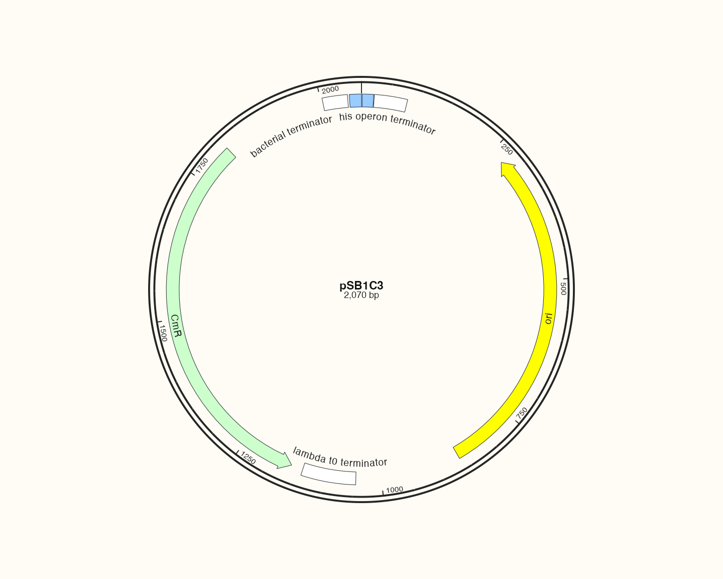
| pSB1C3 | 2070 | 7 |
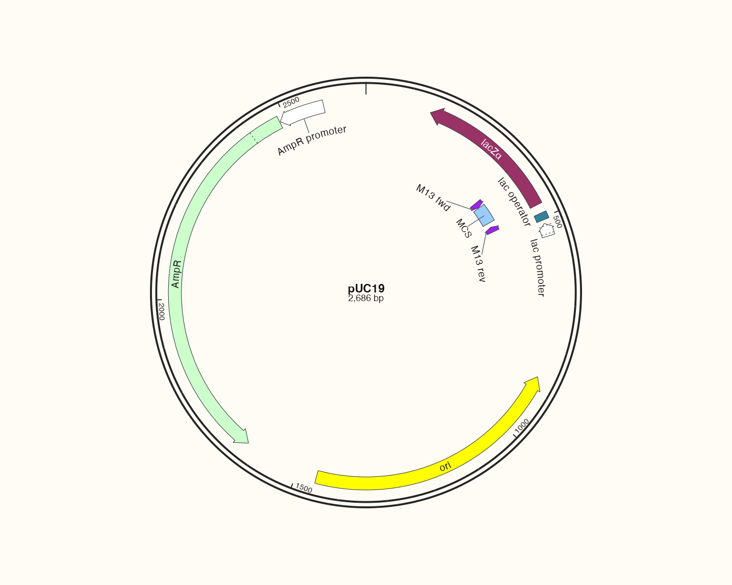
| pUC19 | 2686 | 9 |
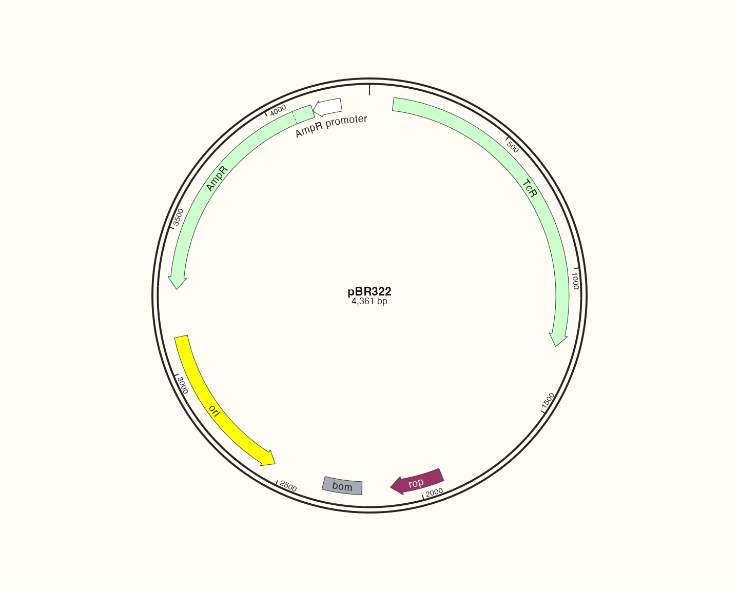
| pBR322 | 4361 | 6 |
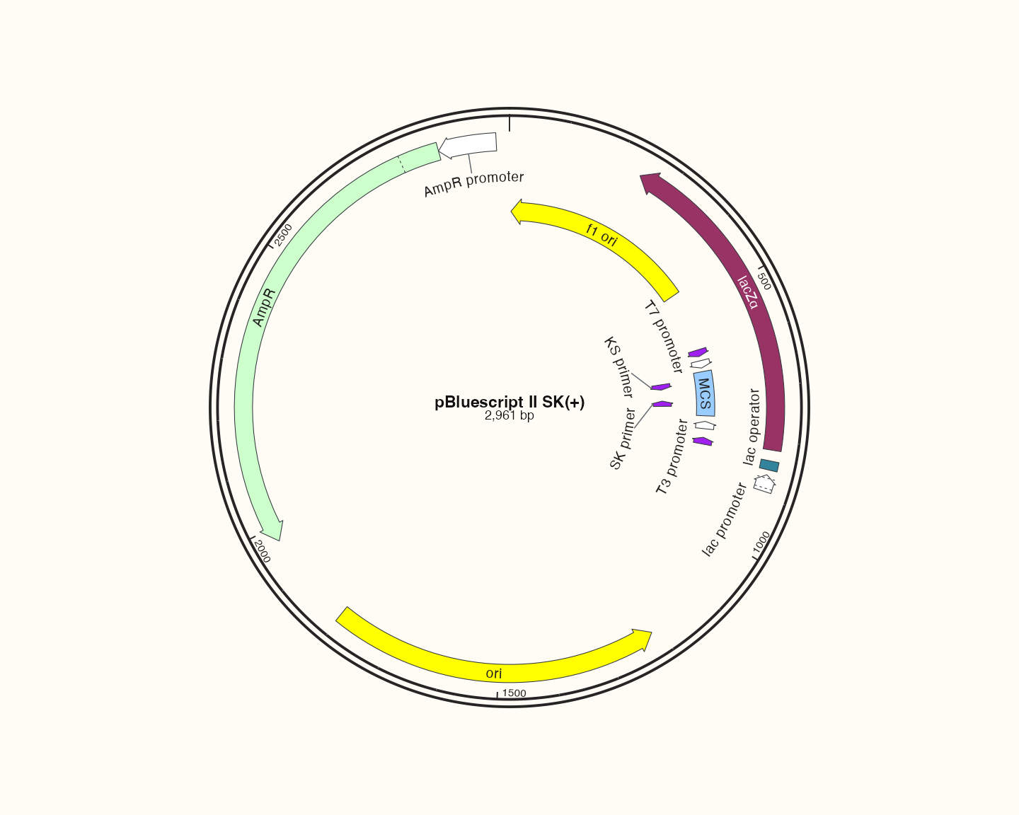
| pBluescript II SK(+) | 2961 | 14 |
| pET-28a(+) | 5369 | 16 |
| pETDuet-1 | 5420 | 20 |
| pDONR221 | 4761 | 11 |
| pcDNA3.1(+) | 5428 | 13 |
| pTRE-Tight-BI | 2856 | 15 |
| pTRIPZ | 13320 | 33 |
| pCAMBIA1300 | 8959 | 17 |
| pEarleyGate 201 | 11779 | 21 |
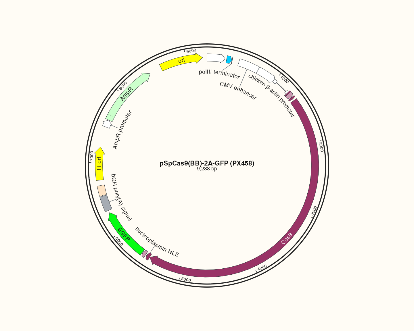
| pSpCas9(BB)-2A-GFP (PX458) | 9288 | 19 |
pSB1C3:小载体与基本骨架
pUC19:常见注释与复制起点
pBR322:多个抗性区与方向
pBluescript II SK(+):局部调控与短特征
pET-28a(+):表达区与标签
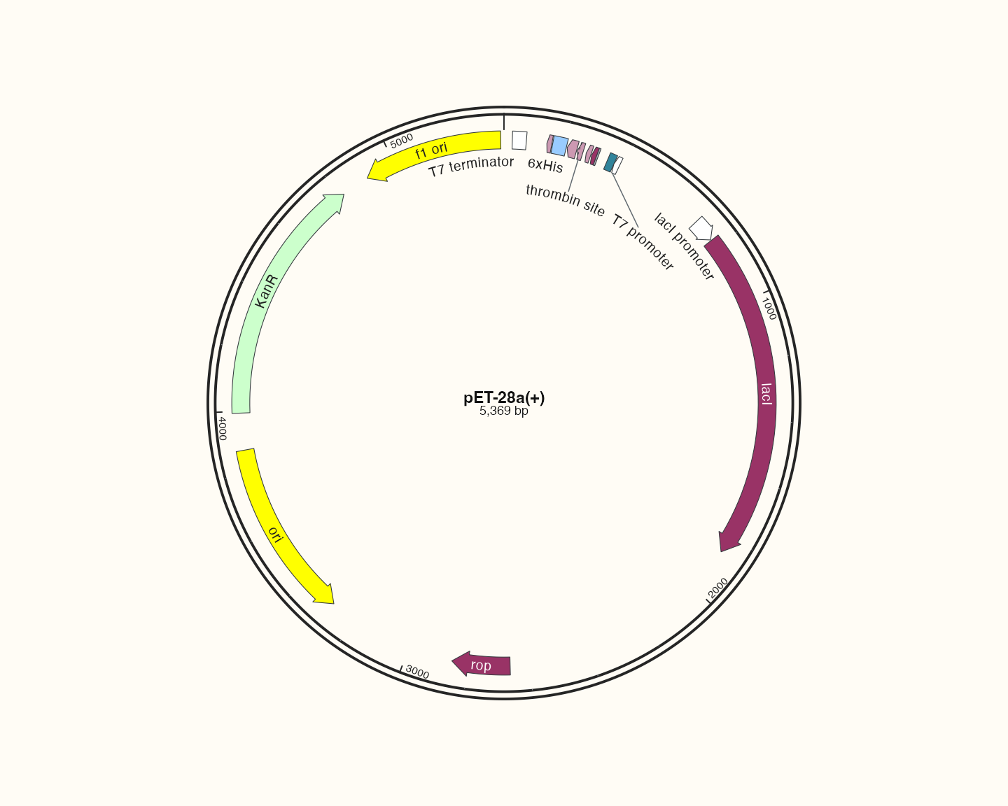
pETDuet-1:双表达单元,进入密集案例
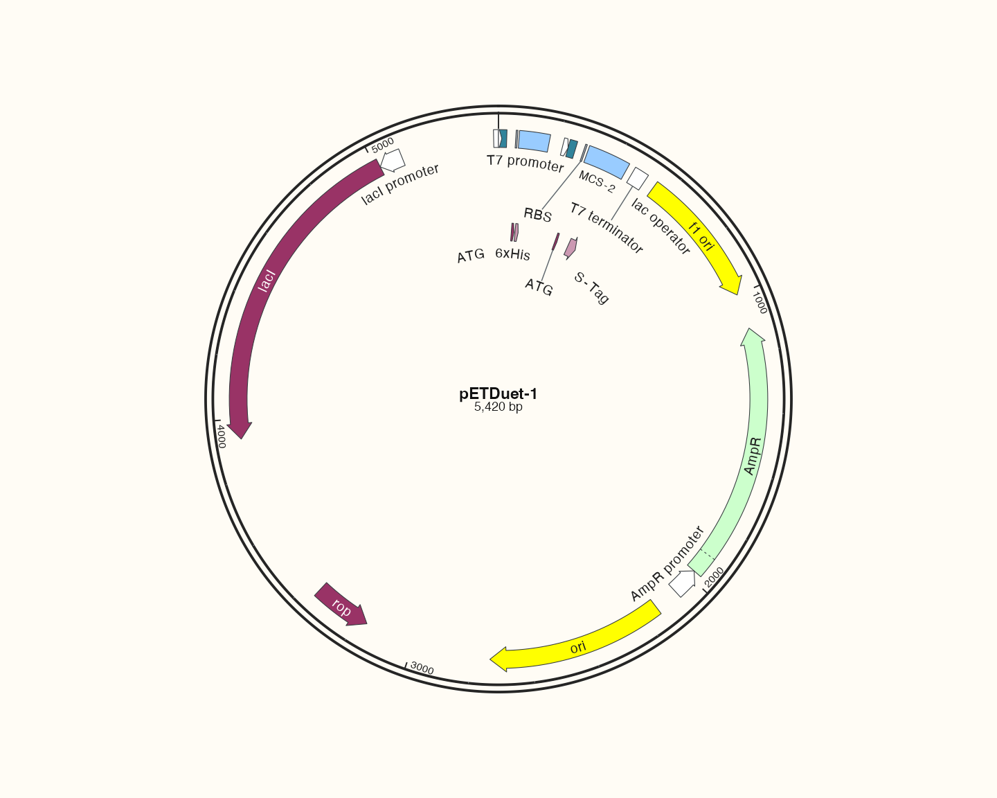
pDONR221:重组相关结构
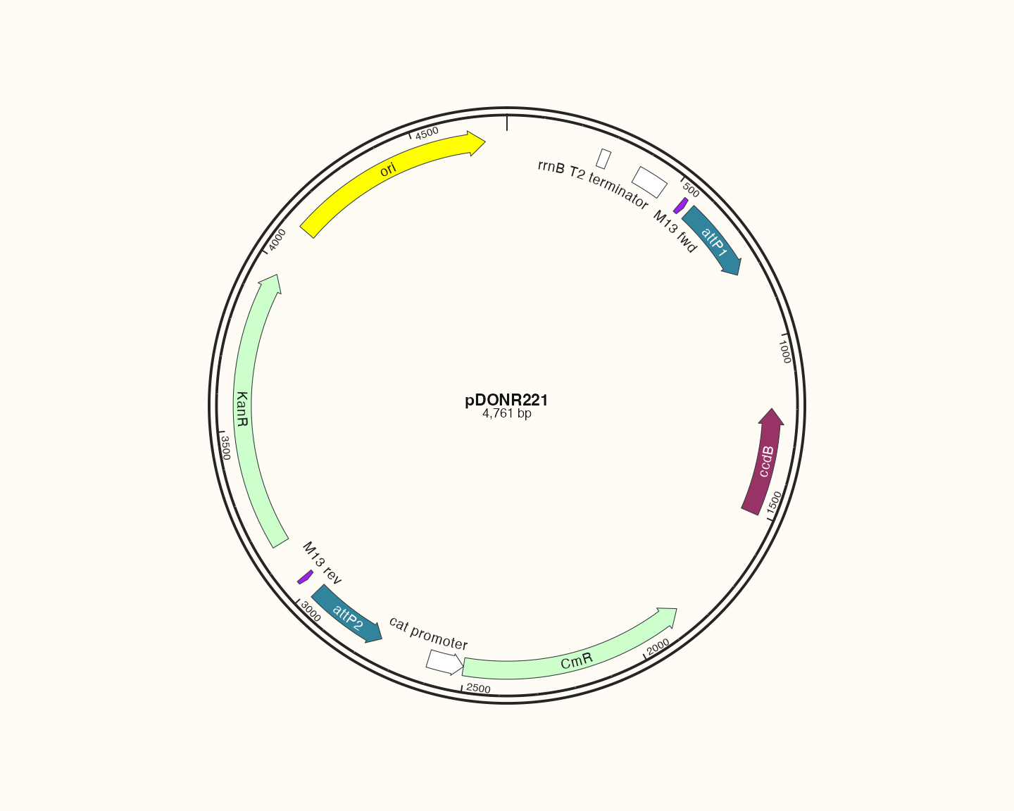
pcDNA3.1(+):表达载体的注释层级
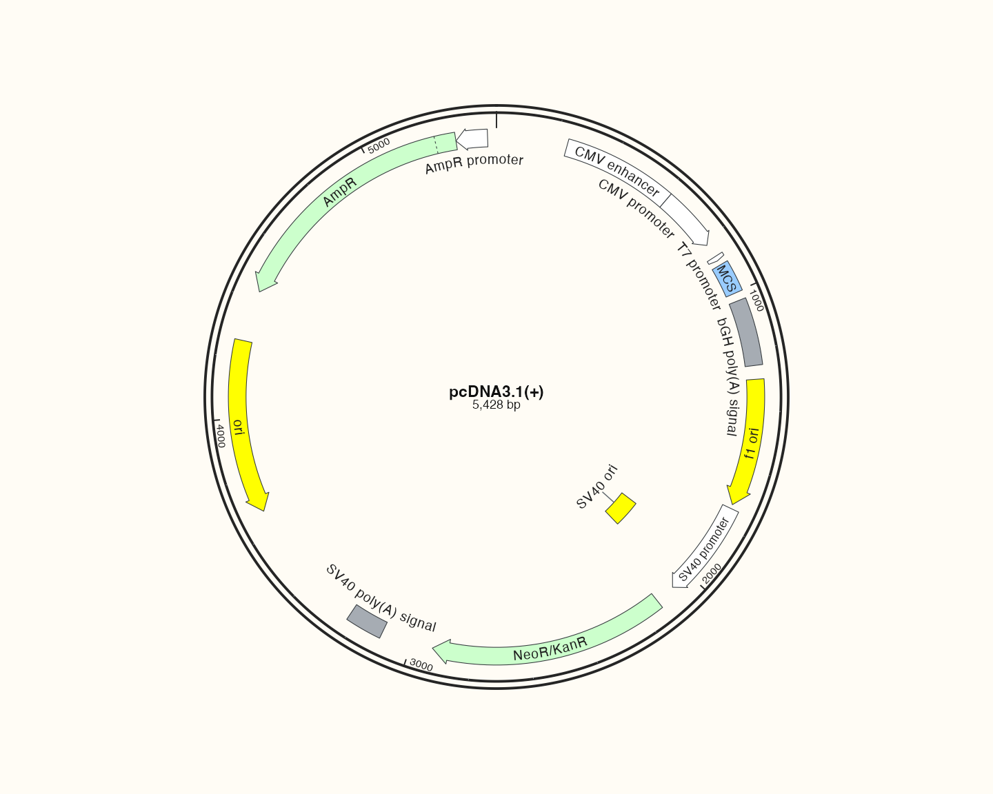
pTRE-Tight-BI:双向调控布局
pTRIPZ:更长序列的显示密度
pCAMBIA1300:较大植物载体的结构
pEarleyGate 201:另一植物载体的类别对照
pSpCas9(BB)-2A-GFP (PX458):大型表达载体与文字适配
下一步
比较不同密度后,进入3.5 综合实战,添加独立引物与酶切图层。