0.16.6 文档
全站目录 · 按任务查找
1.3 从骨架逐层添加
先完成每个小步骤,再查看综合图。四步复用同一组数据,直接比较每次新增图层的作用。
本页准备
先解压教学输入。准备代码 · 在本页运行一次
代码
# Optional appearance choices; none of these columns or scales is required input.
library(ggchord)
seq_palette <- setNames(
  c("#E64B35", "#233E4A", "#269B82", "#D59B17"),
  c("MT108731.1", "MT118296.1", "OQ646790.1", "OR222515.1")
)
gene_palette <- c("+" = "#CE1536", "-" = "#346B9D", "." = "#8291A6")

library(ggchord)
doc_background <- "#FFFCF5"
identity_palette <- c("#303B71", "#36537D", "#269B82", "#A5D52C", "#ECEB31")
identity_values <- c(0, 0.5, 0.8, 0.9, 1)
identity_breaks <- c(0, 50, 80, 90, 100)
doc_legend_theme <- theme(
  legend.title = element_text(size = 13, face = "bold"),
  legend.text = element_text(size = 11),
  legend.key.width = unit(9, "mm"), legend.key.height = unit(5, "mm"),
  legend.spacing.x = unit(9, "mm"), legend.spacing.y = unit(7, "mm"),
  legend.margin = margin(l = 4, r = 4, unit = "mm")
)
sequence_guide <- guide_ggchord_legend(nrow = 1, theme = doc_legend_theme)
strand_guide <- guide_ggchord_legend(
  nrow = 1, override.aes = list(strand = c("+", "-")), theme = doc_legend_theme
)
identity_guide <- guide_ggchord_colourbar(
  position = "left", direction = "vertical",
  theme = theme(
    legend.key.height = unit(75, "mm"), legend.key.width = unit(5, "mm"),
    legend.title = element_text(size = 13, face = "bold"),
    legend.text = element_text(size = 11), legend.margin = margin(r = 7, unit = "mm")
  )
)
doc_theme <- theme_ggchord_publication(
  axis.text = element_text(size = 11),
  axis.text.check.overlap = TRUE
) +
  theme(
    legend.position = "bottom",
    legend.title = element_text(size = 13, face = "bold"),
    legend.text = element_text(size = 11),
    legend.key.width = unit(9, "mm"), legend.key.height = unit(5, "mm"),
    legend.spacing.x = unit(9, "mm"), legend.spacing.y = unit(7, "mm"),
    legend.box.spacing = unit(6, "mm"),
    plot.background = element_rect(fill = doc_background, colour = NA),
    panel.background = element_blank(),
    plot.title = element_text(face = "bold", size = 18),
    plot.subtitle = element_text(size = 10, colour = "#5C625A"),
    plot.margin = margin(14, 18, 14, 18)
  )
doc_axis <- function(coordinates = "relative") {
  scale_seq_position_continuous(
    coordinates = coordinates, n.breaks = 3, minor_breaks = NULL,
    labels = function(x) format(x, scientific = FALSE, big.mark = ",", trim = TRUE)
  )
}

library(ggchord)
library(dplyr)
library(purrr)
library(tidyr)
# Original repository records; extract the tutorial input bundle first.
show_sequences <- read_fasta_lengths(files = "examples/fasta/*.fna") |>
  select(accver, length)
show_annotations <- read_gff3(files = "examples/gff3/*.gff3", unstranded = "keep")
show_genes <- show_annotations |>
  filter(type == "CDS") |>
  select(accver, start, end, strand, anno)
show_alignments <- read_blast(files = "examples/blastn-standard/*.tsv")
# At most three substantial observed HSPs per pair; no coordinates are invented.
show_links <- show_alignments |>
  filter(length >= 900, pident >= 75) |>
  group_by(qaccver, saccver) |>
  slice_max(length, n = 3, with_ties = FALSE) |>
  ungroup()
# Select up to four source CDS per sequence, spread across annotation order.
# No feature is moved or invented; keep complete source tables separately.
show_features <- show_genes |>
  filter(end - start + 1 >= 500) |>
  group_by(accver) |>
  arrange(start, .by_group = TRUE) |>
  mutate(display_bin = ntile(row_number(), 4), informative = !is.na(anno) & anno != "hypothetical protein") |>
  group_by(accver, display_bin) |>
  arrange(desc(informative), desc(end - start), .by_group = TRUE) |>
  slice_head(n = 1) |>
  ungroup() |>
  select(accver, start, end, strand, anno)
# Also retain well-separated negative-strand CDS, if not already represented.
show_reverse <- show_genes |>
  filter(strand == "-", end - start + 1 >= 500) |>
  group_by(accver) |>
  arrange(start, .by_group = TRUE) |>
  slice(c(1, n())) |>
  ungroup()
show_features <- bind_rows(show_features, show_reverse) |>
  distinct(accver, start, end, strand, .keep_all = TRUE) |>
  arrange(accver, start)
show_labels <- show_features
show_optimization <- optimize_ggchord_layout(
  show_sequences, show_links,
  optimize = "orientation", weight = "length"
)
第一步:只有序列骨架
代码
p_learn_seq <- ggchord(seq_data = show_sequences) +
  geom_seq() +
  geom_seq_label(size = 4) +
  scale_seq_colour_manual(
    values = seq_palette, name = "Sequence",
    guide = sequence_guide
  ) +
  scale_seq_position_continuous(breaks = c(0, 20000, 40000), minor_breaks = NULL) +
  coord_chord() +
  doc_theme
p_learn_seq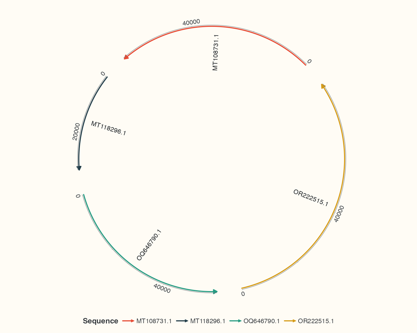
geom_seq() 画骨架,geom_seq_label() 标识序列,coord_chord() 选择整体视图;此时不需要连接或基因输入。
第二步:加入已有比对
代码
p_learn_links <- p_learn_seq +
  geom_link_ribbon(
    aes(ribbon_fill = pident),
    data = show_links,
    adjacent_only = FALSE, link_avoid = "smooth"
  ) +
  scale_ribbon_fill_gradientn(
    colours = identity_palette, values = identity_values, limits = c(0, 100),
    breaks = identity_breaks, name = "Identity (%)", guide = identity_guide
  )
p_learn_links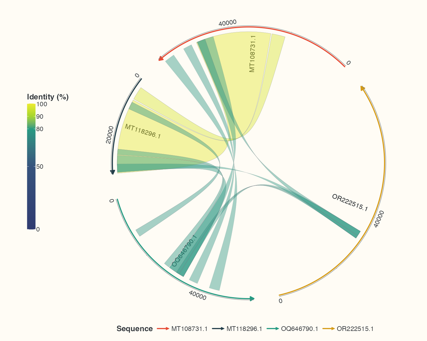
相似度由aes和scale表达;显式保留非相邻连接,让后面替换坐标时仍使用相同的连接数据。
第三步:加入精选基因
代码
p_learn_genes <- p_learn_links +
  geom_gene(data = show_features, position = position_strand(0.08)) +
  scale_gene_fill_manual(values = gene_palette, breaks = c("+", "-"), name = "Strand") +
  guides(gene_fill = strand_guide)
p_learn_genes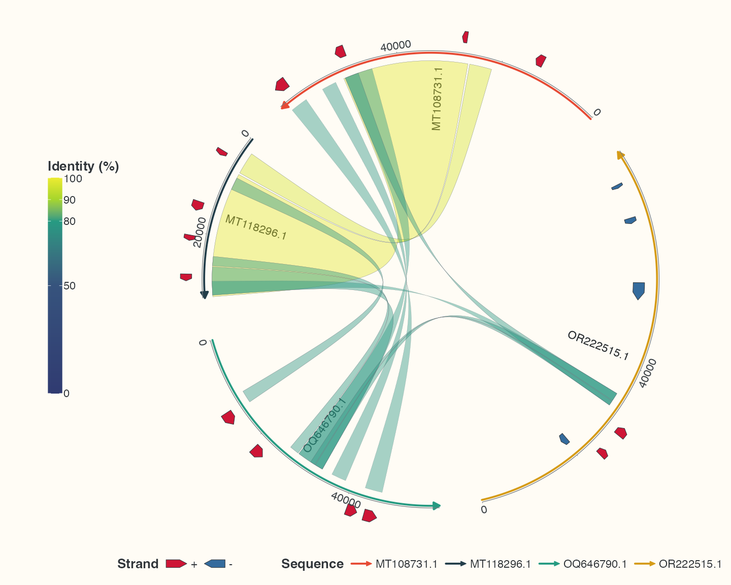
position_strand() 将正负链分到骨架两侧。仅展示真实筛选的注释,原表仍保留全部CDS。
第四步:给每个展示特征加标签
代码
p_learn_labels <- p_learn_genes +
  geom_gene_label_repel(
    data = show_features, label_layout = "arc", label_wrap = 24,
    label_max_lines = 3, position = position_strand(0.08), size = 3
  )
p_learn_labels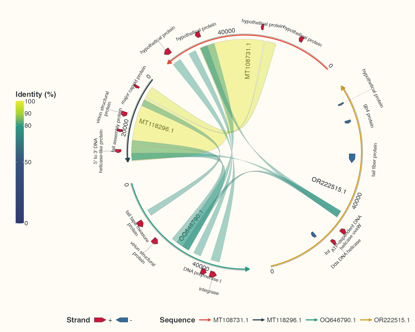
同一特征表交给箭头层与repel标签层;标签层不另行筛选。与单独添加图层相比,改名、删行或排序会改变业务含义,应保留明确中间对象。
继续:1.4 方向、半径、曲率和避障。