0.16.6 documentation

Site guide · find your task

Setup and learning paths

HomeInstall and prepare the environmentChoose your learning module

Module I · Chord

1.1 Tables and field meanings1.2 Produce and import comparisons1.3 Build the layers step by step1.4 Direction, curvature and clearance1.5 Filter and summarize links1.6 Full source-file workflow1.7 Complete chord showcase

Module II · Collinear

2.1 Reuse chord input tables2.2 Switch coordinates and add layers2.3 Routes, clearance and the ruler2.4 Compare CDS neighbourhoods2.5 Focus, anchors and segments2.6 Complete collinear showcase

Module III · Plasmid

3.1 DNA, annotations and 13 references3.2 From a circle to annotation layers3.3 Features, primers and restriction3.4 Thirteen plasmid references3.5 Complete plasmid cases

Consult as needed · Data and layers

Prepare tables and coordinatesImport and convert dataImport nucleotide and protein alignmentsProject protein intervals to genomic coordinatesFeatures, stacking and genomic decorationLabels and local placementQuantitative tracksMappings, scales, guides and themesSet values by sequence and strandCommon adjustments and grammarExport, preview and diagnostics

Learning map and reference

Articles and complete workflowsFunction referenceReproducible galleryFrequently asked questionsMigrate to the candidate APITerminology and design sourcesDevelopment status and changes

2.4 Compare CDS neighbourhoods

On this page

• Prepare this page
• 1. Extract actual CDS and coding DNA
• 2. Declare members and sequence pairs
• 3. Focus on comparable neighbourhoods
• 4. Project supported protein intervals to both CDS
• Check your result
• Save this result

Compare AmpR neighbourhoods in two plasmids. Check real coding DNA, establish correspondence, then focus to each CDS plus 200 bp on either side.

Prepare this page

Only bundled data is needed; no download or new alignment. Load the package and optional display settings first.

Preparation code — run once on this page

Code

library(ggchord)
doc_background <- "#FFFCF5"
identity_palette <- c("#303B71", "#36537D", "#269B82", "#A5D52C", "#ECEB31")
identity_values <- c(0, 0.5, 0.8, 0.9, 1)
identity_breaks <- c(0, 50, 80, 90, 100)
doc_legend_theme <- theme(
  legend.title = element_text(size = 13, face = "bold"),
  legend.text = element_text(size = 11),
  legend.key.width = unit(9, "mm"), legend.key.height = unit(5, "mm"),
  legend.spacing.x = unit(9, "mm"), legend.spacing.y = unit(7, "mm"),
  legend.margin = margin(l = 4, r = 4, unit = "mm")
)
sequence_guide <- guide_ggchord_legend(nrow = 1, theme = doc_legend_theme)
strand_guide <- guide_ggchord_legend(
  nrow = 1, override.aes = list(strand = c("+", "-")), theme = doc_legend_theme
)
identity_guide <- guide_ggchord_colourbar(
  position = "left", direction = "vertical",
  theme = theme(
    legend.key.height = unit(75, "mm"), legend.key.width = unit(5, "mm"),
    legend.title = element_text(size = 13, face = "bold"),
    legend.text = element_text(size = 11), legend.margin = margin(r = 7, unit = "mm")
  )
)
doc_theme <- theme_ggchord_publication(
  axis.text = element_text(size = 11),
  axis.text.check.overlap = TRUE
) +
  theme(
    legend.position = "bottom",
    legend.title = element_text(size = 13, face = "bold"),
    legend.text = element_text(size = 11),
    legend.key.width = unit(9, "mm"), legend.key.height = unit(5, "mm"),
    legend.spacing.x = unit(9, "mm"), legend.spacing.y = unit(7, "mm"),
    legend.box.spacing = unit(6, "mm"),
    plot.background = element_rect(fill = doc_background, colour = NA),
    panel.background = element_blank(),
    plot.title = element_text(face = "bold", size = 18),
    plot.subtitle = element_text(size = 10, colour = "#5C625A"),
    plot.margin = margin(14, 18, 14, 18)
  )
doc_axis <- function(coordinates = "relative") {
  scale_seq_position_continuous(
    coordinates = coordinates, n.breaks = 3, minor_breaks = NULL,
    labels = function(x) format(x, scientific = FALSE, big.mark = ",", trim = TRUE)
  )
}

1. Extract actual CDS and coding DNA

Select AmpR annotations from bundled pUC19 and pETDuet-1, retaining IDs, coordinates, strand and text. Reverse-complement negative-strand DNA so comparisons use the same biological orientation rather than annotation names alone.

Code

library(dplyr)
data(plasmid_example_pUC19)
data(plasmid_example_pETDuet_1)
homolog_source <- bind_rows(plasmid_example_pUC19, plasmid_example_pETDuet_1)
homolog_seq <- homolog_source |>
  select(accver, length)
cluster_features <- homolog_source |>
  find_common_features() |>
  filter(type == "CDS", anno == "AmpR") |>
  select(accver, start, end, strand, anno) |>
  arrange(match(accver, homolog_source$accver)) |>
  mutate(feature_id = paste(accver, start, end, sep = ":"))
# Membership is computed from exact strand-corrected CDS DNA equality, not gene names.
reverse_complement <- function(sequence) {
  bases <- strsplit(sequence, "")[[1]]
  chartr("ACGT", "TGCA", paste(rev(bases), collapse = ""))
}
coding_sequences <- cluster_features |>
  left_join(select(homolog_source, accver, sequence), by = "accver") |>
  rowwise() |>
  mutate(
    coding_dna = substr(sequence, start, end),
    coding_dna = if (strand == "-") reverse_complement(coding_dna) else coding_dna
  ) |>
  ungroup()
cds_dna <- pull(coding_sequences, coding_dna)

cluster_features should contain two actual CDS; cds_dna retains their oriented coding sequences. This strict example checks exact DNA equality. General homology analysis can use external alignments and clustering; homologs need not be identical.

2. Declare members and sequence pairs

Build membership from exact coding-DNA equality. Different DNA does not enter one group merely because both annotations say AmpR.

Code

membership <- tibble(
  feature_id = cluster_features$feature_id,
  cluster_id = paste0("exact_CDS_", match(cds_dna, unique(cds_dna)))
)
homologs <- link_ggchord_clusters(cluster_features, membership,
  pairs = tibble(qaccver = homolog_seq$accver[1], saccver = homolog_seq$accver[2])
)
loci <- find_ggchord_loci(homolog_seq, cluster_features,
  targets = cluster_features$feature_id[cluster_features$anno == "AmpR"][1], upstream = 100, downstream = 100
)

Inspect membership and homologs$report$comparisons and $members. The linking utility consumes existing groups; it does not compute a new alignment. Unknown members and ambiguous paralogs are reported; only explicit paralogs = "all" requests all combinations within the documented bounds.

3. Focus on comparable neighbourhoods

Full plasmid lengths would shrink the individual CDS. Construct windows from each real CDS source interval and add 200 bp on either side, retaining the original sequence and annotation tables.

Code

# Compare equivalent local windows instead of shrinking one gene on full plasmids.
homolog_windows <- cluster_features |>
  select(accver, start, end)
local_homologs <- focus_ggchord_data(homolog_seq, homologs$data, cluster_features,
  loci = homolog_windows, expand = 200
)
p_homologs <- ggchord(
  seq_data = local_homologs$seq_data,
  ribbon_data = local_homologs$ribbon_data, gene_data = local_homologs$gene_data
) +
  geom_link_ribbon(fill = "#269B82", alpha = .65) +
  geom_seq(colour = "#233E4A", show.legend = FALSE) +
  geom_feature(
    data = local_homologs$gene_data, feature_fill = "#F1D334",
    position = position_strand(.10), width = .07
  ) +
  geom_feature_label_repel(data = local_homologs$gene_data, size = 4, label_fit = "shrink") +
  geom_seq_label(size = 4) +
  geom_seq_break() +
  coord_collinear() +
  doc_axis("source") +
  doc_theme
p_homologs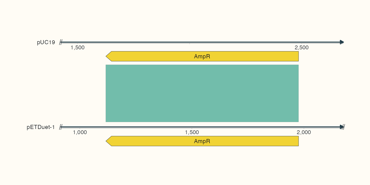

AmpR neighbourhoods: identical CDS, 200 bp flanks and source coordinates · Click to enlarge

Gold arrows identify the checked identical coding sequences; the purple band connects their CDS ranges and internal text names AmpR. Axes use each original sequence’s positions, so one horizontal location can have different source labels. Break markers indicate that only local windows remain.

local_homologs$report records retention and clipping. Genes outside the windows are omitted, not absent. The band represents declared interval correspondence, not a base alignment; envelopes of segmented annotations likewise do not establish exon-level correspondence.

4. Project supported protein intervals to both CDS

Code

# Exact CDS DNA equality supplies evidence for these selected ungapped residues.
matching <- homologs$data |>
  slice_head(n = 1)
paired_coding <- cluster_features |>
  mutate(phase = 0)
paired_cds <- build_ggchord_cds(paired_coding)
protein_link <- tibble(
  qfeature_id = matching$qfeature_id, sfeature_id = matching$sfeature_id,
  qstart = 1, qend = 20, sstart = 1, send = 20
)
projected_links <- project_ggchord_links(protein_link, paired_cds, ungapped = TRUE)
projected_links

Metric	Observed output
Projected genomic feature rows	1
Projected nucleotide link rows	1

The first 20 residues of identical CDS provide sequence evidence for ungapped = TRUE. Equal spans alone do not justify that claim for ordinary BLASTp HSPs. The utility retains protein statistics rather than presenting them as nucleotide identity.

Check your result

Both internal labels should read AmpR and arrows retain the actual negative strand. Coding DNA supports correspondence; source axes and focus reports explain the local display. Save at explicit 10 × 5 in dimensions.

Next: read real BLASTp query intervals, understand CDS projection and segments, or create independent local windows.

Save this result

Save the plot just created to the working directory; use matching dimensions for preview.

Code

ggsave("ampR-neighbourhood.png", p_homologs, width = 10, height = 5, units = "in", dpi = 144)