Site guide · find your task
2.5 Focus, anchors and segments
On this page
Select local windows or segments while keeping source positions distinct from display transformations.
Prepare this page
In a fresh R session, run the code below, then follow this page in order. Colours and layout are optional display choices; inputs select only the fields needed.
Preparation code — run once on this page
Code
library(ggchord)
library(dplyr)
data(seq_data_example)
data(ribbon_data_example)
data(gene_data_example)
seqs <- seq_data_example |>
  select(accver, length)
links <- ribbon_data_example |>
  select(qaccver, saccver, qstart, qend, sstart, send)
# The fixture preserves biological strands separately from its old display strands.
genes <- gene_data_example |>
  transmute(accver, start, end, strand = source_strand)

# Optional appearance choices; none of these columns or scales is required input.
library(ggchord)
seq_palette <- setNames(
  c("#E64B35", "#233E4A", "#269B82", "#D59B17"),
  c("MT108731.1", "MT118296.1", "OQ646790.1", "OR222515.1")
)
gene_palette <- c("+" = "#CE1536", "-" = "#346B9D", "." = "#8291A6")

library(ggchord)
doc_background <- "#FFFCF5"
identity_palette <- c("#303B71", "#36537D", "#269B82", "#A5D52C", "#ECEB31")
identity_values <- c(0, 0.5, 0.8, 0.9, 1)
identity_breaks <- c(0, 50, 80, 90, 100)
doc_legend_theme <- theme(
  legend.title = element_text(size = 13, face = "bold"),
  legend.text = element_text(size = 11),
  legend.key.width = unit(9, "mm"), legend.key.height = unit(5, "mm"),
  legend.spacing.x = unit(9, "mm"), legend.spacing.y = unit(7, "mm"),
  legend.margin = margin(l = 4, r = 4, unit = "mm")
)
sequence_guide <- guide_ggchord_legend(nrow = 1, theme = doc_legend_theme)
strand_guide <- guide_ggchord_legend(
  nrow = 1, override.aes = list(strand = c("+", "-")), theme = doc_legend_theme
)
identity_guide <- guide_ggchord_colourbar(
  position = "left", direction = "vertical",
  theme = theme(
    legend.key.height = unit(75, "mm"), legend.key.width = unit(5, "mm"),
    legend.title = element_text(size = 13, face = "bold"),
    legend.text = element_text(size = 11), legend.margin = margin(r = 7, unit = "mm")
  )
)
doc_theme <- theme_ggchord_publication(
  axis.text = element_text(size = 11),
  axis.text.check.overlap = TRUE
) +
  theme(
    legend.position = "bottom",
    legend.title = element_text(size = 13, face = "bold"),
    legend.text = element_text(size = 11),
    legend.key.width = unit(9, "mm"), legend.key.height = unit(5, "mm"),
    legend.spacing.x = unit(9, "mm"), legend.spacing.y = unit(7, "mm"),
    legend.box.spacing = unit(6, "mm"),
    plot.background = element_rect(fill = doc_background, colour = NA),
    panel.background = element_blank(),
    plot.title = element_text(face = "bold", size = 18),
    plot.subtitle = element_text(size = 10, colour = "#5C625A"),
    plot.margin = margin(14, 18, 14, 18)
  )
doc_axis <- function(coordinates = "relative") {
  scale_seq_position_continuous(
    coordinates = coordinates, n.breaks = 3, minor_breaks = NULL,
    labels = function(x) format(x, scientific = FALSE, big.mark = ",", trim = TRUE)
  )
}
Focus without losing origins
After this page’s preparation code:
Code
focus_loci <- tibble(
  accver = seqs$accver,
  start = floor(seqs$length * .25), end = floor(seqs$length * .75)
)
focused <- focus_ggchord_data(seqs, links, genes, loci = focus_loci)
p_focus <- ggchord(
  seq_data = focused$seq_data, ribbon_data = focused$ribbon_data,
  gene_data = focused$gene_data
) +
  geom_seq() +
  geom_link_ribbon(fill = "#6BAFA6", alpha = .5) +
  geom_gene() +
  geom_seq_break() +
  geom_seq_label(size = 4) +
  scale_seq_colour_manual(values = seq_palette) +
  scale_gene_fill_manual(values = gene_palette) +
  doc_axis("source") +
  coord_collinear() +
  doc_theme
p_focus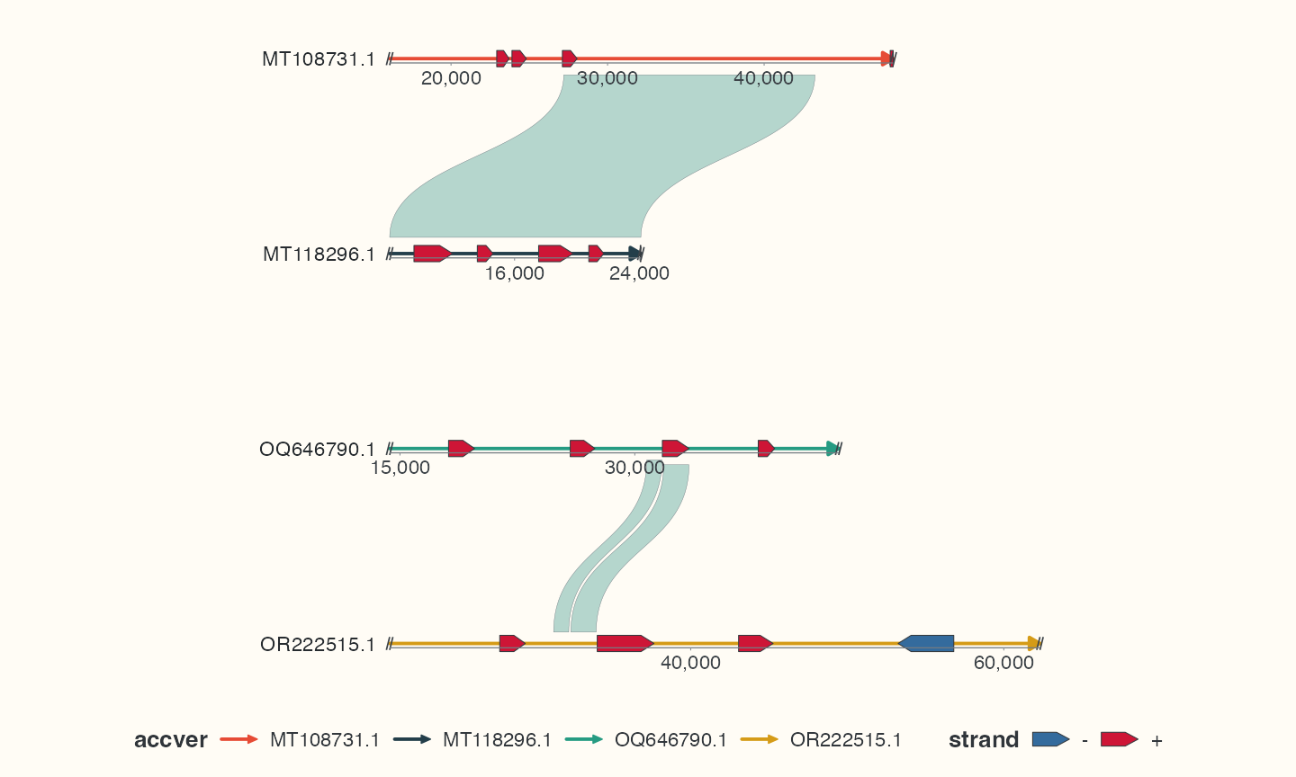
Focus relocates retained positions to local one-based coordinates and retains source origins, truncation flags and a report. boundary = "trim" can clip links by a linear display projection; it does not realign sequences. A scaled alignment length is flagged as estimated. coordinates = "source" restores source axis labels, including after repeated focusing.
Independent windows and local reversal
Code
windows <- tibble(
  accver = rep(seqs$accver[1], 2),
  start = c(1, floor(seqs$length[1] * .65)), end = c(floor(seqs$length[1] * .4), seqs$length[1]),
  locus_id = c("left_window", "right_window"), row_id = seqs$accver[1], orientation = c(1, -1)
)
segmented <- segment_ggchord_data(slice_head(seqs, n = 1), windows = windows)
p_segments <- ggchord(seq_data = segmented$seq_data) +
  geom_seq() +
  coord_collinear(segments = segmented$segments, segment_gap = 2000)
p_segments
Each window has a reversible source mapping; omitted gaps have no mapping. map_ggchord_position() maps explicit source positions into a plot for ordinary ggplot2 annotations. Supply the window ID when windows share a source sequence. Do not interpret display orientation as a change to the original strand.
Explicit biological relationships
find_ggchord_loci() selects declared feature/name queries. link_ggchord_clusters() requires an explicit membership table and sequence pairs; equal gene names do not establish homology. filter_ggchord_ribbons(), deduplicate_ggchord_ribbons() and merge_ggchord_ribbons() prepare existing alignments, preserving source membership and estimated-length flags. Bundle and density statistics summarize provided links rather than creating new sequence alignments.
Map an annotation back to source coordinates
Code
source_position <- focus_loci$start[1] + 100
source_mark <- map_ggchord_position(p_focus, seqs$accver[1], source_position, source = TRUE)
p_marked <- p_focus +
  ggplot2::geom_point(
    data = source_mark, aes(x, y),
    inherit.aes = FALSE, colour = "#D59B17", size = 3
  )
p_marked
Run the focus example first. The helper returns Cartesian x/y for a source position 100 bp inside the first selected window. It does not make all ordinary ggplot2 coordinates become genomic bp. In segmented views choose the window ID, and check positions in omitted gaps rather than extrapolating across them. Use explicit homologs when the locus selection comes from declared feature/cluster evidence.
Check your result
Inspect cropping reports, break markers and source coordinates. Omitted gaps have no mapping; a display flip alone is not evidence of inversion.