Site guide · find your task
1.3 Build the layers step by step
On this page
Complete each small step before the flagship example. All four views reuse the same records, making the effect of each added layer visible.
Prepare this page
Extract the input bundle first.Preparation code — run once on this page
Code
# Optional appearance choices; none of these columns or scales is required input.
library(ggchord)
seq_palette <- setNames(
  c("#E64B35", "#233E4A", "#269B82", "#D59B17"),
  c("MT108731.1", "MT118296.1", "OQ646790.1", "OR222515.1")
)
gene_palette <- c("+" = "#CE1536", "-" = "#346B9D", "." = "#8291A6")

library(ggchord)
doc_background <- "#FFFCF5"
identity_palette <- c("#303B71", "#36537D", "#269B82", "#A5D52C", "#ECEB31")
identity_values <- c(0, 0.5, 0.8, 0.9, 1)
identity_breaks <- c(0, 50, 80, 90, 100)
doc_legend_theme <- theme(
  legend.title = element_text(size = 13, face = "bold"),
  legend.text = element_text(size = 11),
  legend.key.width = unit(9, "mm"), legend.key.height = unit(5, "mm"),
  legend.spacing.x = unit(9, "mm"), legend.spacing.y = unit(7, "mm"),
  legend.margin = margin(l = 4, r = 4, unit = "mm")
)
sequence_guide <- guide_ggchord_legend(nrow = 1, theme = doc_legend_theme)
strand_guide <- guide_ggchord_legend(
  nrow = 1, override.aes = list(strand = c("+", "-")), theme = doc_legend_theme
)
identity_guide <- guide_ggchord_colourbar(
  position = "left", direction = "vertical",
  theme = theme(
    legend.key.height = unit(75, "mm"), legend.key.width = unit(5, "mm"),
    legend.title = element_text(size = 13, face = "bold"),
    legend.text = element_text(size = 11), legend.margin = margin(r = 7, unit = "mm")
  )
)
doc_theme <- theme_ggchord_publication(
  axis.text = element_text(size = 11),
  axis.text.check.overlap = TRUE
) +
  theme(
    legend.position = "bottom",
    legend.title = element_text(size = 13, face = "bold"),
    legend.text = element_text(size = 11),
    legend.key.width = unit(9, "mm"), legend.key.height = unit(5, "mm"),
    legend.spacing.x = unit(9, "mm"), legend.spacing.y = unit(7, "mm"),
    legend.box.spacing = unit(6, "mm"),
    plot.background = element_rect(fill = doc_background, colour = NA),
    panel.background = element_blank(),
    plot.title = element_text(face = "bold", size = 18),
    plot.subtitle = element_text(size = 10, colour = "#5C625A"),
    plot.margin = margin(14, 18, 14, 18)
  )
doc_axis <- function(coordinates = "relative") {
  scale_seq_position_continuous(
    coordinates = coordinates, n.breaks = 3, minor_breaks = NULL,
    labels = function(x) format(x, scientific = FALSE, big.mark = ",", trim = TRUE)
  )
}

library(ggchord)
library(dplyr)
library(purrr)
library(tidyr)
# Original repository records; extract the tutorial input bundle first.
show_sequences <- read_fasta_lengths(files = "examples/fasta/*.fna") |>
  select(accver, length)
show_annotations <- read_gff3(files = "examples/gff3/*.gff3", unstranded = "keep")
show_genes <- show_annotations |>
  filter(type == "CDS") |>
  select(accver, start, end, strand, anno)
show_alignments <- read_blast(files = "examples/blastn-standard/*.tsv")
# At most three substantial observed HSPs per pair; no coordinates are invented.
show_links <- show_alignments |>
  filter(length >= 900, pident >= 75) |>
  group_by(qaccver, saccver) |>
  slice_max(length, n = 3, with_ties = FALSE) |>
  ungroup()
# Select up to four source CDS per sequence, spread across annotation order.
# No feature is moved or invented; keep complete source tables separately.
show_features <- show_genes |>
  filter(end - start + 1 >= 500) |>
  group_by(accver) |>
  arrange(start, .by_group = TRUE) |>
  mutate(display_bin = ntile(row_number(), 4), informative = !is.na(anno) & anno != "hypothetical protein") |>
  group_by(accver, display_bin) |>
  arrange(desc(informative), desc(end - start), .by_group = TRUE) |>
  slice_head(n = 1) |>
  ungroup() |>
  select(accver, start, end, strand, anno)
# Also retain well-separated negative-strand CDS, if not already represented.
show_reverse <- show_genes |>
  filter(strand == "-", end - start + 1 >= 500) |>
  group_by(accver) |>
  arrange(start, .by_group = TRUE) |>
  slice(c(1, n())) |>
  ungroup()
show_features <- bind_rows(show_features, show_reverse) |>
  distinct(accver, start, end, strand, .keep_all = TRUE) |>
  arrange(accver, start)
show_labels <- show_features
show_optimization <- optimize_ggchord_layout(
  show_sequences, show_links,
  optimize = "orientation", weight = "length"
)
Step 1: sequence backbones
Code
p_learn_seq <- ggchord(seq_data = show_sequences) +
  geom_seq() +
  geom_seq_label(size = 4) +
  scale_seq_colour_manual(
    values = seq_palette, name = "Sequence",
    guide = sequence_guide
  ) +
  scale_seq_position_continuous(breaks = c(0, 20000, 40000), minor_breaks = NULL) +
  coord_chord() +
  doc_theme
p_learn_seq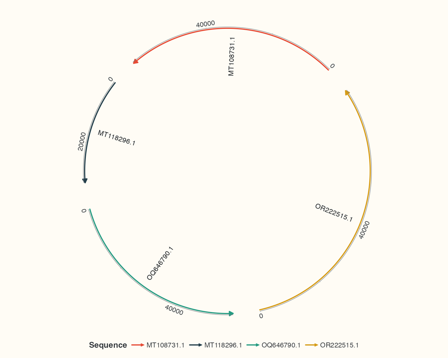
geom_seq() draws backbones, geom_seq_label() identifies sequences, and coord_chord() selects the global view. No links or genes are required yet.
Step 2: observed comparisons
Code
p_learn_links <- p_learn_seq +
  geom_link_ribbon(
    aes(ribbon_fill = pident),
    data = show_links,
    adjacent_only = FALSE, link_avoid = "smooth"
  ) +
  scale_ribbon_fill_gradientn(
    colours = identity_palette, values = identity_values, limits = c(0, 100),
    breaks = identity_breaks, name = "Identity (%)", guide = identity_guide
  )
p_learn_links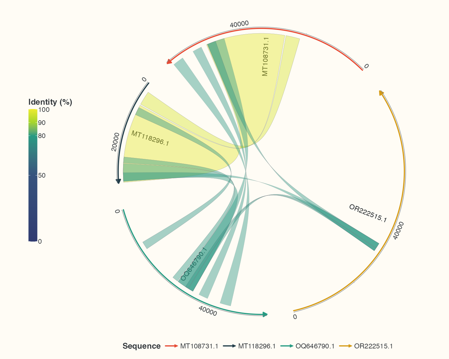
Identity belongs in aes and a scale. Explicitly retaining non-neighbour links keeps the same link data when replacing coordinates later.
Step 3: selected genes
Code
p_learn_genes <- p_learn_links +
  geom_gene(data = show_features, position = position_strand(0.08)) +
  scale_gene_fill_manual(values = gene_palette, breaks = c("+", "-"), name = "Strand") +
  guides(gene_fill = strand_guide)
p_learn_genes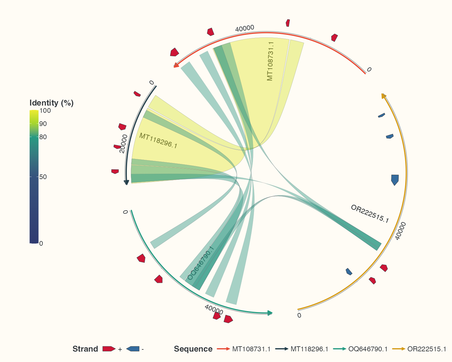
position_strand() separates positive and negative strands. Display selected real annotations while retaining every source CDS separately.
Step 4: label every displayed feature
Code
p_learn_labels <- p_learn_genes +
  geom_gene_label_repel(
    data = show_features, label_layout = "arc", label_wrap = 24,
    label_max_lines = 3, position = position_strand(0.08), size = 3
  )
p_learn_labels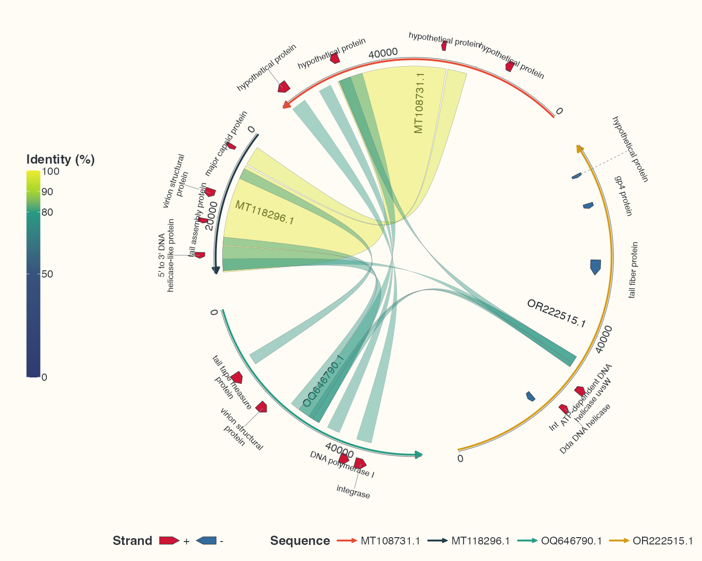
The arrow and repel-label layers receive the same feature table without another label filter. Renaming, deleting or reordering records can change meaning; retain clear intermediate objects.
Continue to 1.4 Direction, radius, curvature and clearance.