Site guide · find your task
Labels and local placement
On this page
Arrange text while retaining annotation geometry: choose export dimensions and a label subset before choosing automatic or fixed placement.
Prepare this page
In a fresh R session, run the code below, then follow this page in order. Colours and layout are optional display choices; inputs select only the fields needed.
Preparation code — run once on this page
Code
library(ggchord)
library(dplyr)
data(seq_data_example)
data(ribbon_data_example)
data(gene_data_example)
seqs <- seq_data_example |>
  select(accver, length)
links <- ribbon_data_example |>
  select(qaccver, saccver, qstart, qend, sstart, send)
# The fixture preserves biological strands separately from its old display strands.
genes <- gene_data_example |>
  transmute(accver, start, end, strand = source_strand)

# Optional appearance choices; none of these columns or scales is required input.
library(ggchord)
seq_palette <- setNames(
  c("#E64B35", "#233E4A", "#269B82", "#D59B17"),
  c("MT108731.1", "MT118296.1", "OQ646790.1", "OR222515.1")
)
gene_palette <- c("+" = "#CE1536", "-" = "#346B9D", "." = "#8291A6")

library(ggchord)
doc_background <- "#FFFCF5"
identity_palette <- c("#303B71", "#36537D", "#269B82", "#A5D52C", "#ECEB31")
identity_values <- c(0, 0.5, 0.8, 0.9, 1)
identity_breaks <- c(0, 50, 80, 90, 100)
doc_legend_theme <- theme(
  legend.title = element_text(size = 13, face = "bold"),
  legend.text = element_text(size = 11),
  legend.key.width = unit(9, "mm"), legend.key.height = unit(5, "mm"),
  legend.spacing.x = unit(9, "mm"), legend.spacing.y = unit(7, "mm"),
  legend.margin = margin(l = 4, r = 4, unit = "mm")
)
sequence_guide <- guide_ggchord_legend(nrow = 1, theme = doc_legend_theme)
strand_guide <- guide_ggchord_legend(
  nrow = 1, override.aes = list(strand = c("+", "-")), theme = doc_legend_theme
)
identity_guide <- guide_ggchord_colourbar(
  position = "left", direction = "vertical",
  theme = theme(
    legend.key.height = unit(75, "mm"), legend.key.width = unit(5, "mm"),
    legend.title = element_text(size = 13, face = "bold"),
    legend.text = element_text(size = 11), legend.margin = margin(r = 7, unit = "mm")
  )
)
doc_theme <- theme_ggchord_publication(
  axis.text = element_text(size = 11),
  axis.text.check.overlap = TRUE
) +
  theme(
    legend.position = "bottom",
    legend.title = element_text(size = 13, face = "bold"),
    legend.text = element_text(size = 11),
    legend.key.width = unit(9, "mm"), legend.key.height = unit(5, "mm"),
    legend.spacing.x = unit(9, "mm"), legend.spacing.y = unit(7, "mm"),
    legend.box.spacing = unit(6, "mm"),
    plot.background = element_rect(fill = doc_background, colour = NA),
    panel.background = element_blank(),
    plot.title = element_text(face = "bold", size = 18),
    plot.subtitle = element_text(size = 10, colour = "#5C625A"),
    plot.margin = margin(14, 18, 14, 18)
  )
doc_axis <- function(coordinates = "relative") {
  scale_seq_position_continuous(
    coordinates = coordinates, n.breaks = 3, minor_breaks = NULL,
    labels = function(x) format(x, scientific = FALSE, big.mark = ",", trim = TRUE)
  )
}
Select a layout
Gene labels offer "auto", "radial" and "arc" layouts. General feature labels additionally support the internal-first "feature" default and external "callout" layout. Choose the documented values for the layer you use; they are not interchangeable presets.
After this page’s preparation code:
Code
label_data <- gene_data_example |>
  filter(anno != "hypothetical protein") |>
  transmute(accver, start, end, strand = source_strand, anno)
p_labels <- ggchord(seq_data = seqs, gene_data = genes) +
  geom_seq() +
  geom_gene() +
  geom_gene_label_repel(data = label_data, label_layout = "auto", size = 4, label_wrap = 22) +
  geom_seq_label(size = 4) +
  coord_collinear() +
  doc_axis() +
  scale_seq_colour_manual(values = seq_palette) +
  scale_gene_fill_manual(values = gene_palette) +
  doc_theme
p_labels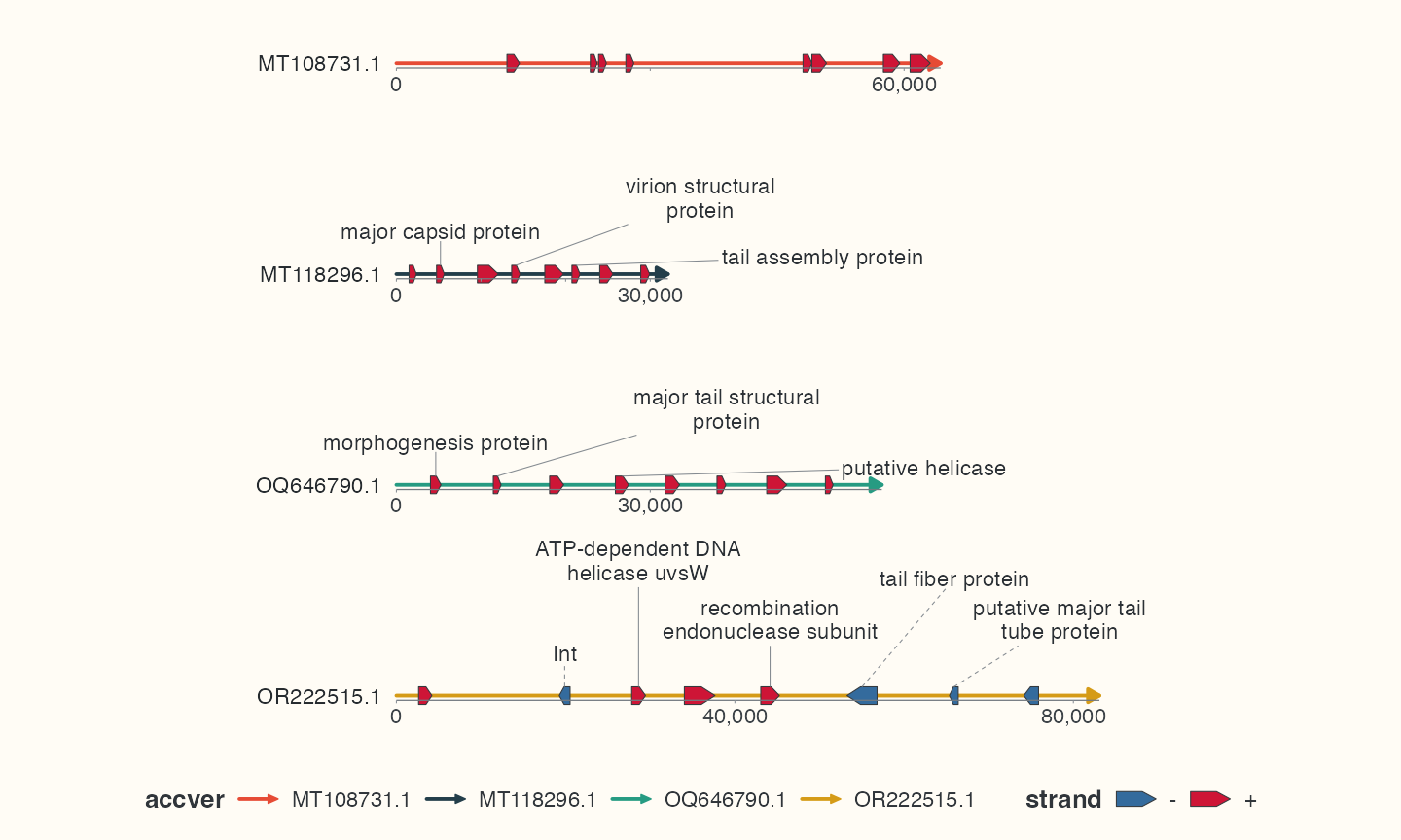
Fixed and automatic placement
Use geom_gene_label() or geom_feature_label() for manual label_rotation, radial/circumferential offsets and orientation controls. Automatic layers reject these manual controls: choose label_layout or remove the manual argument. Use size, colour and family for supported fixed text styles.
label_fit, label_wrap, label_max_lines and label_min_size control fitting where supported. Shrinking is explicit and bounded. Unresolved labels may move or hide; the feature geometry remains. Inspect label_fit_diagnostics and label_diagnostics at the final export size.
Match anchors across layers
In collinear mode, an omitted feature-label Position inherits an unambiguous matching feature layer. Unique feature_id permits reordering or subsets, but accession, interval and strand must agree. Multiple matching layers need an explicit Position or unambiguous IDs. Preview after selecting the final device size; resizing the Plots pane changes the available space.
Compare the three gene layouts
Code
# Compare layouts with at most the first and last informative label per sequence.
comparison_labels <- label_data |>
  group_by(accver) |>
  filter(row_number() %in% c(1L, n())) |>
  ungroup()
label_plots <- lapply(c("auto", "radial", "arc"), function(layout) {
  ggchord(seq_data = seqs, gene_data = genes) +
    geom_seq() +
    geom_gene() +
    geom_gene_label_repel(data = comparison_labels, label_layout = layout, size = 4, label_wrap = 22) +
    geom_seq_label(size = 4) +
    scale_seq_colour_manual(values = seq_palette, name = "Sequence",
      guide = guide_ggchord_legend(nrow = 2, theme = doc_legend_theme)) +
    scale_gene_fill_manual(values = gene_palette, breaks = c("+", "-"), name = "Strand", guide = strand_guide) +
    coord_chord(xlim = c(-1.8, 1.8), ylim = c(-1.6, 1.6)) +
    theme_ggchord_publication(axis = element_blank()) +
    doc_legend_theme +
    theme(
      legend.position = "bottom",
      plot.background = element_rect(fill = doc_background, colour = NA),
      panel.background = element_blank()
    ) +
    labs(title = layout)
})
names(label_plots) <- c("auto", "radial", "arc")
p_manual_labels <- ggchord(seq_data = seqs, gene_data = genes) +
  geom_seq() +
  geom_gene() +
  geom_gene_label(data = label_data, label_rotation = 30) +
  coord_collinear()
label_plots$auto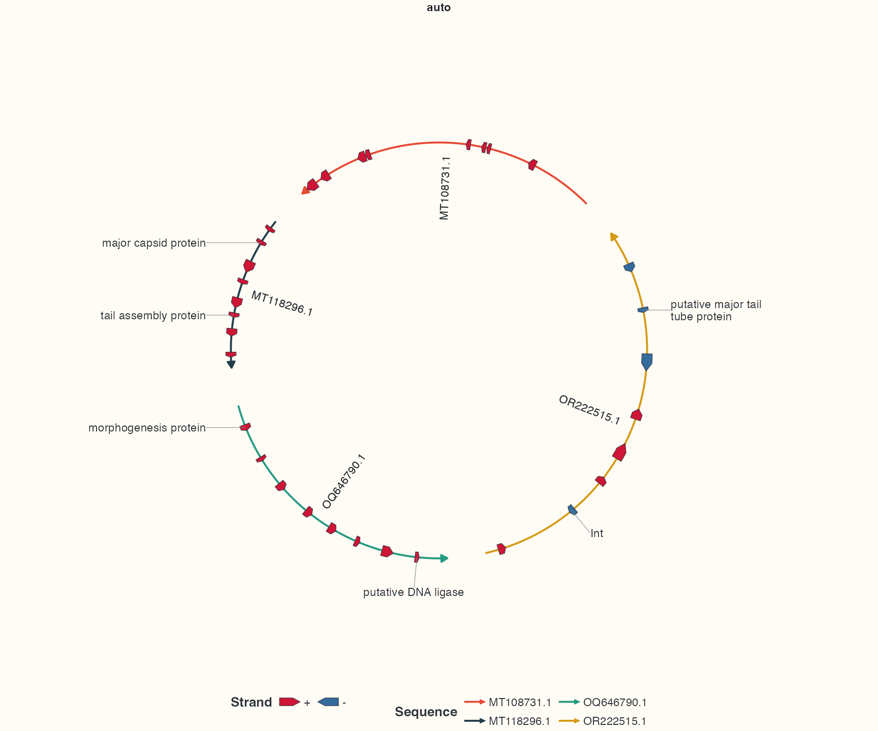
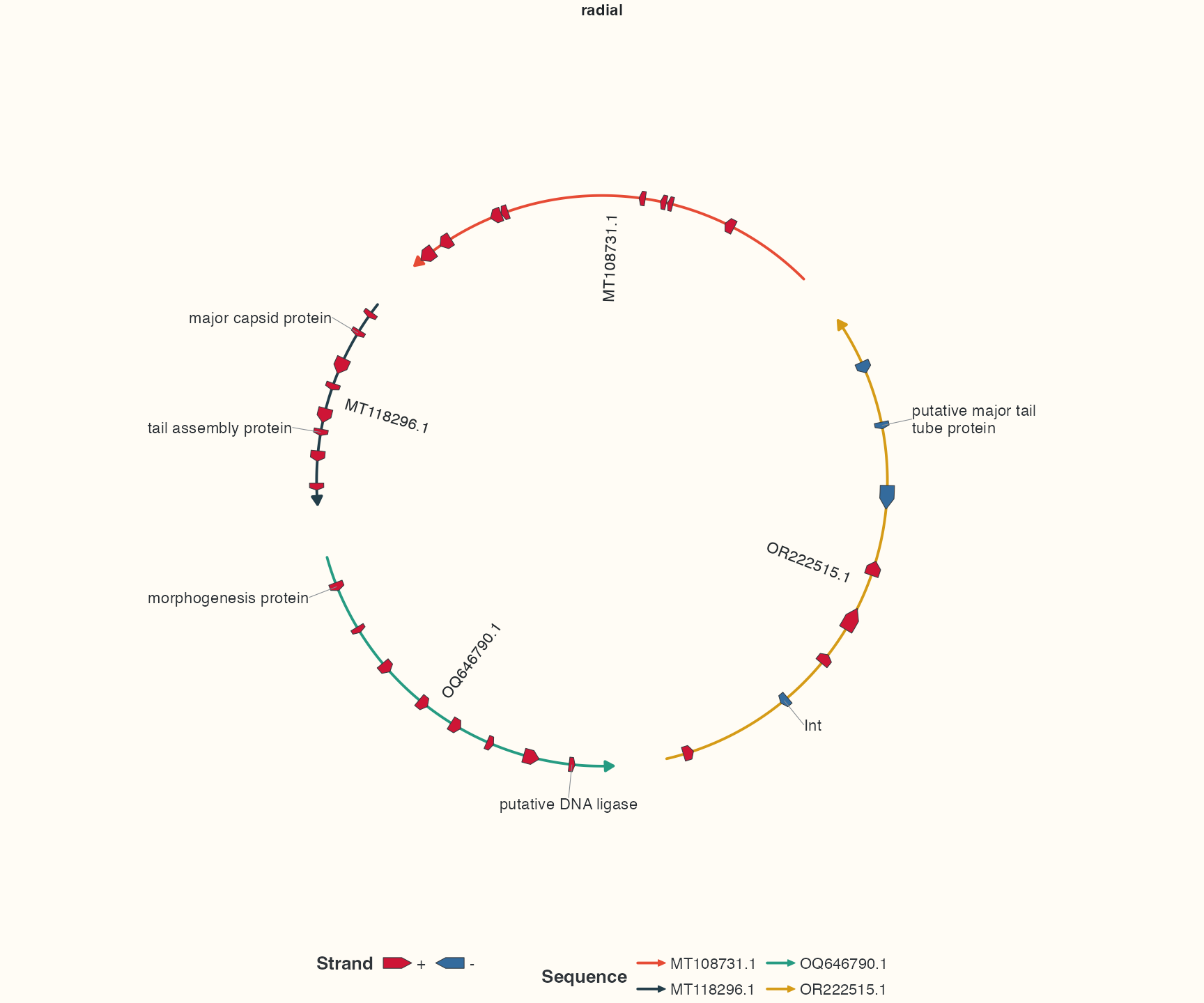
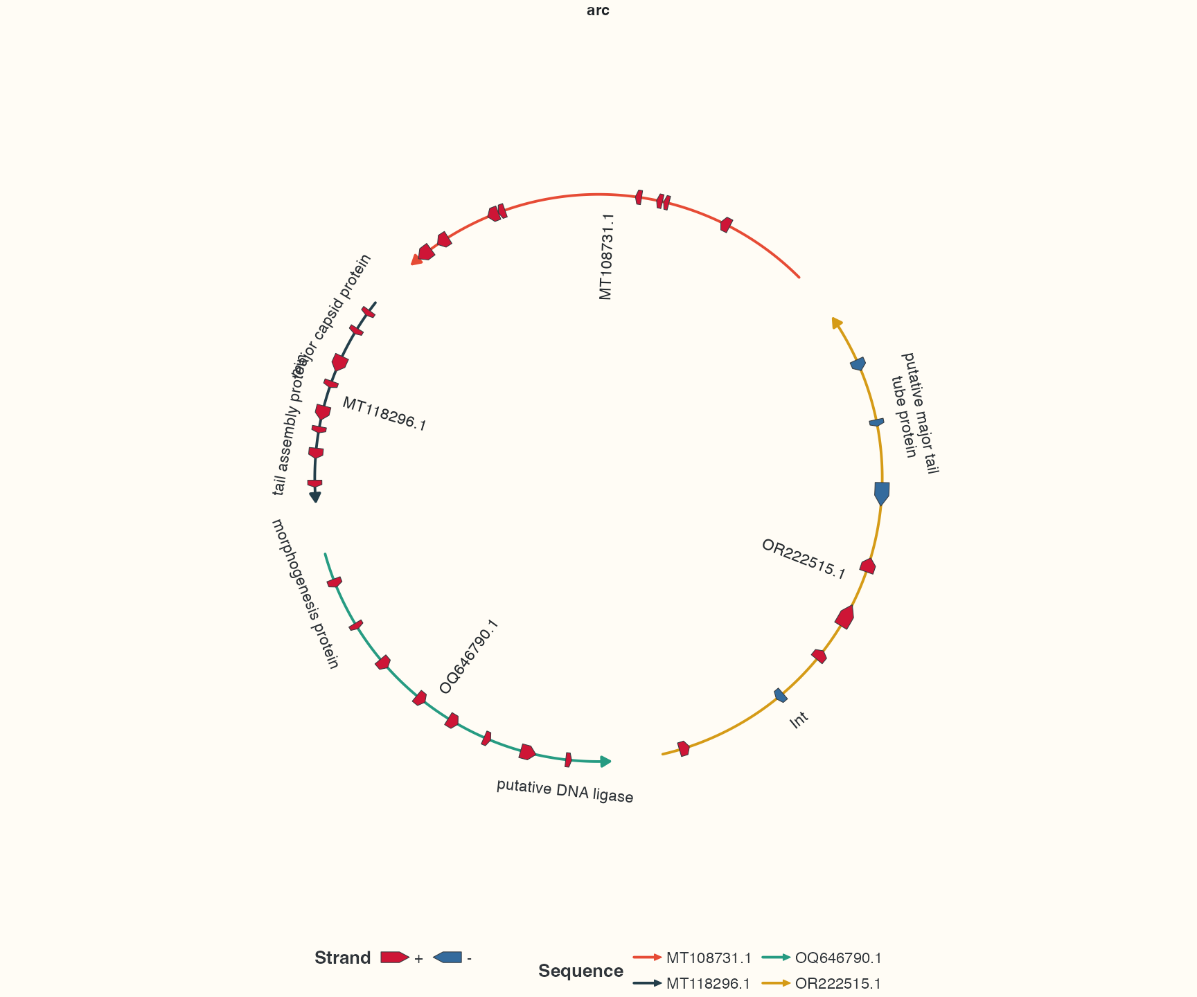
Keep at most the first and last informative labels per sequence, retaining all gene arrows, to compare text orientation. Print label_plots$auto, $radial or $arc to inspect a candidate. The inputs and requested font size are identical; only the layout choice changes. Auto uses shared columns where applicable, radial follows local contours and arc follows the sequence tangent. p_manual_labels shows the separate fixed-label route; its explicit rotation does not belong in an automatic repel layer. General feature labels have additional internal-first/callout choices; see the complete circular workflow for dense mixed annotation and stacking for inherited or explicit Position anchors.
Check your result
The three layout comparisons share the same input. Assess text direction, leaders and hiding reasons together; missing text does not mean a feature was lost.