3.4 Thirteen plasmid references

On this page

Prepare all cases once
Inputs and recognition results
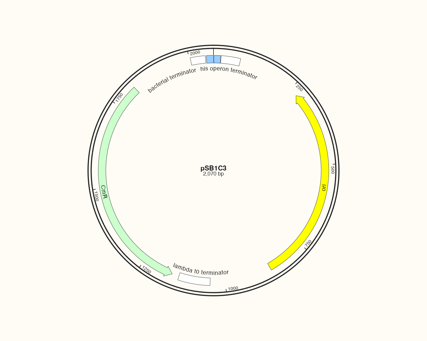
pSB1C3: Small vector and basic structure
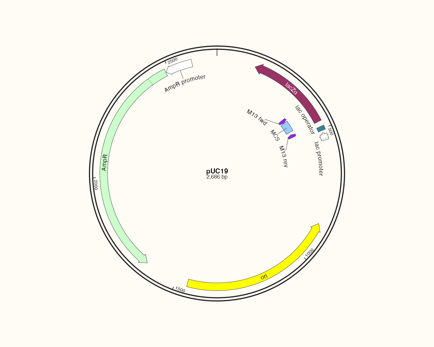
pUC19: Common features and replication origin
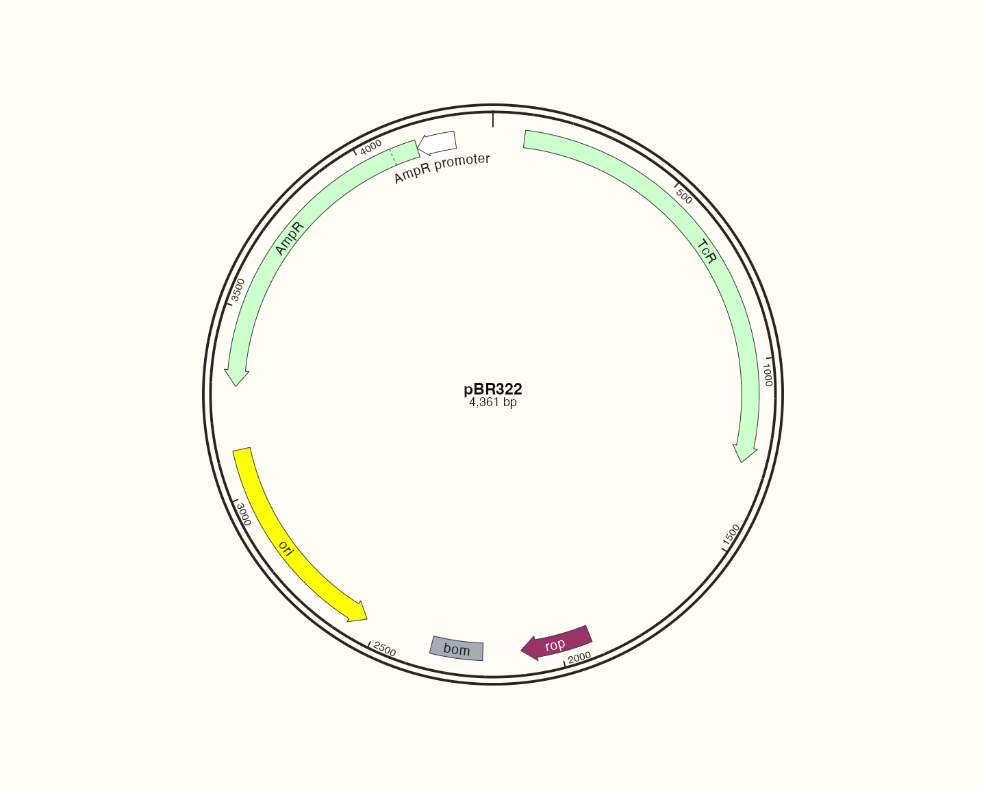
pBR322: Multiple resistance regions and direction
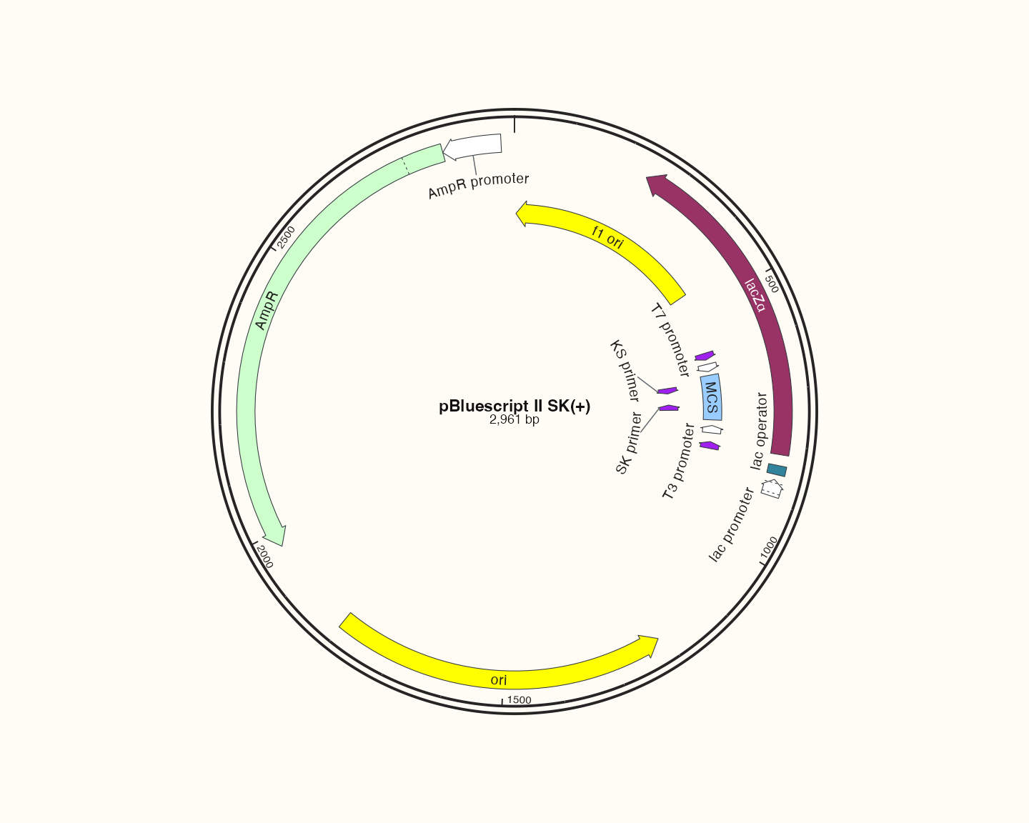
pBluescript II SK(+): Local regulation and short features
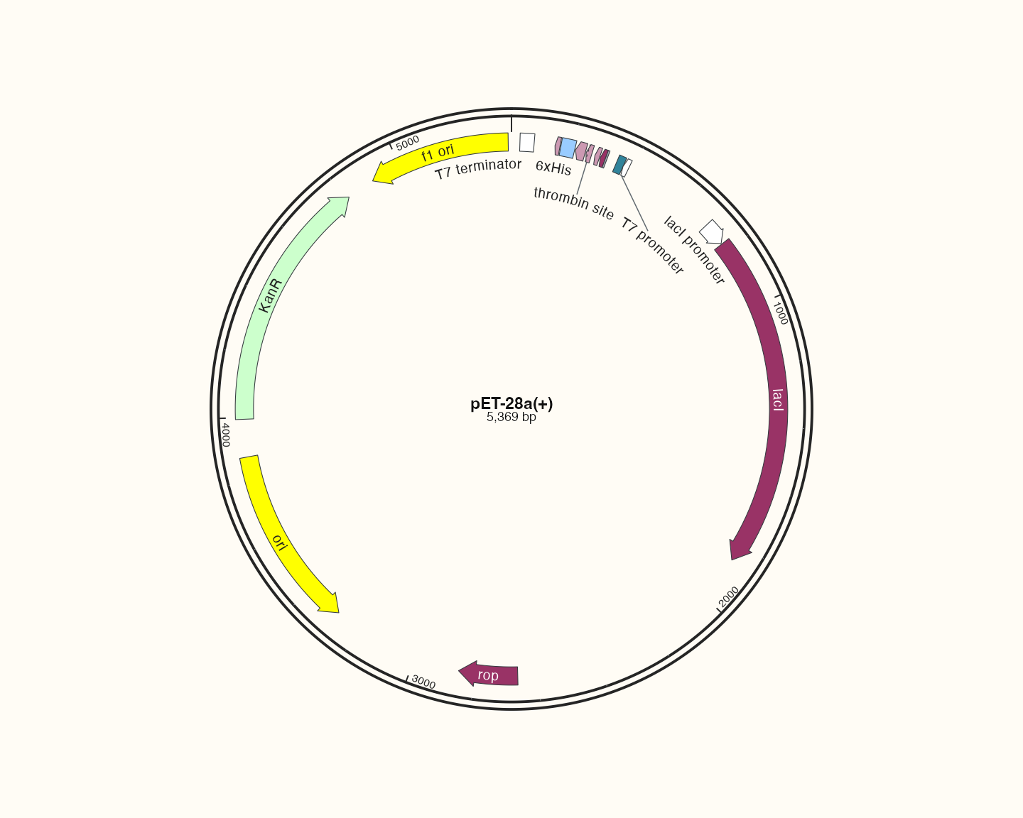
pET-28a(+): Expression regions and tags
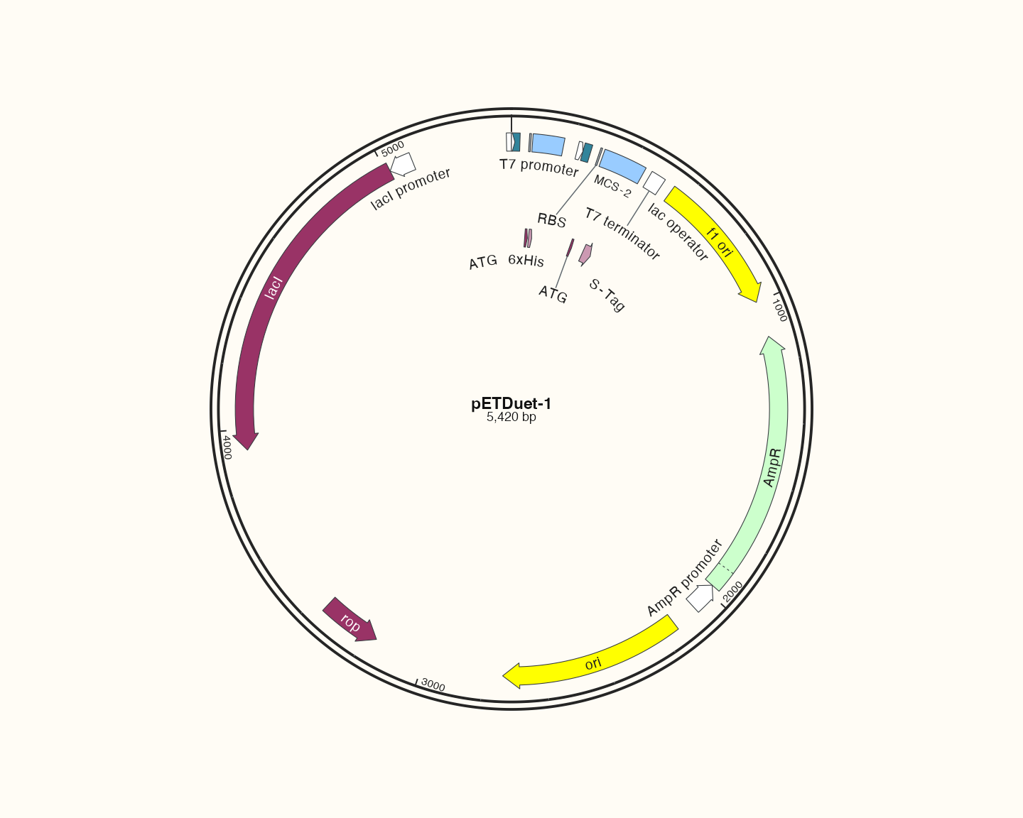
pETDuet-1: Dual expression units; transition to the dense case
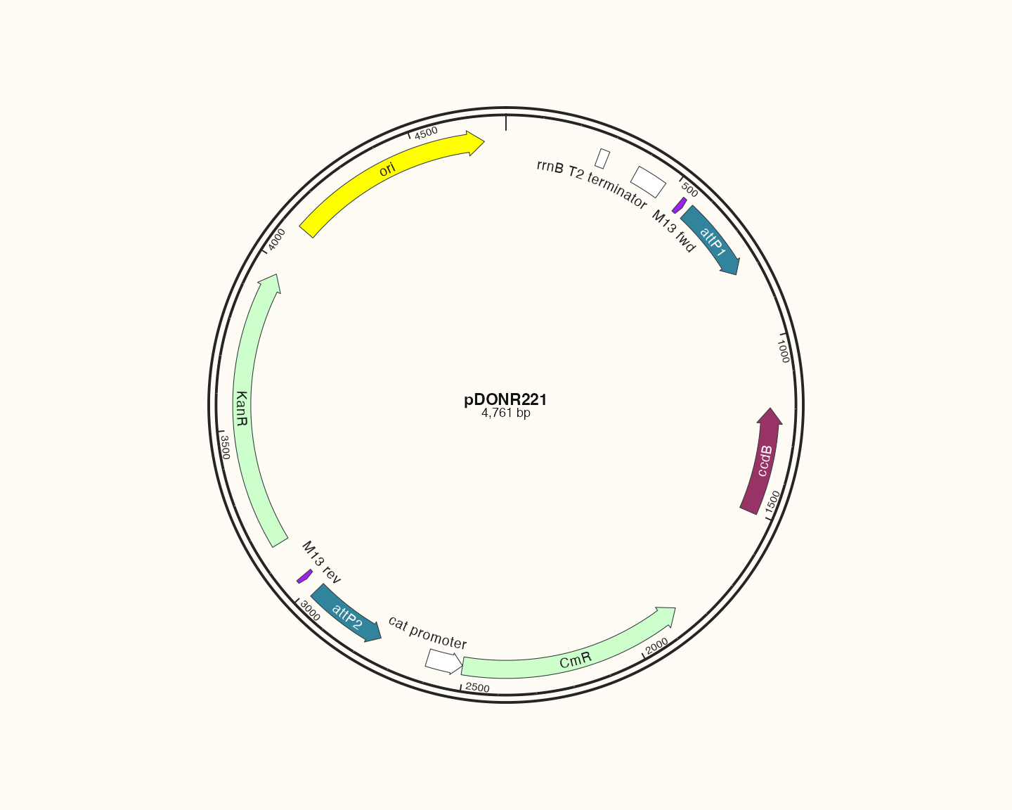
pDONR221: Recombination-related architecture
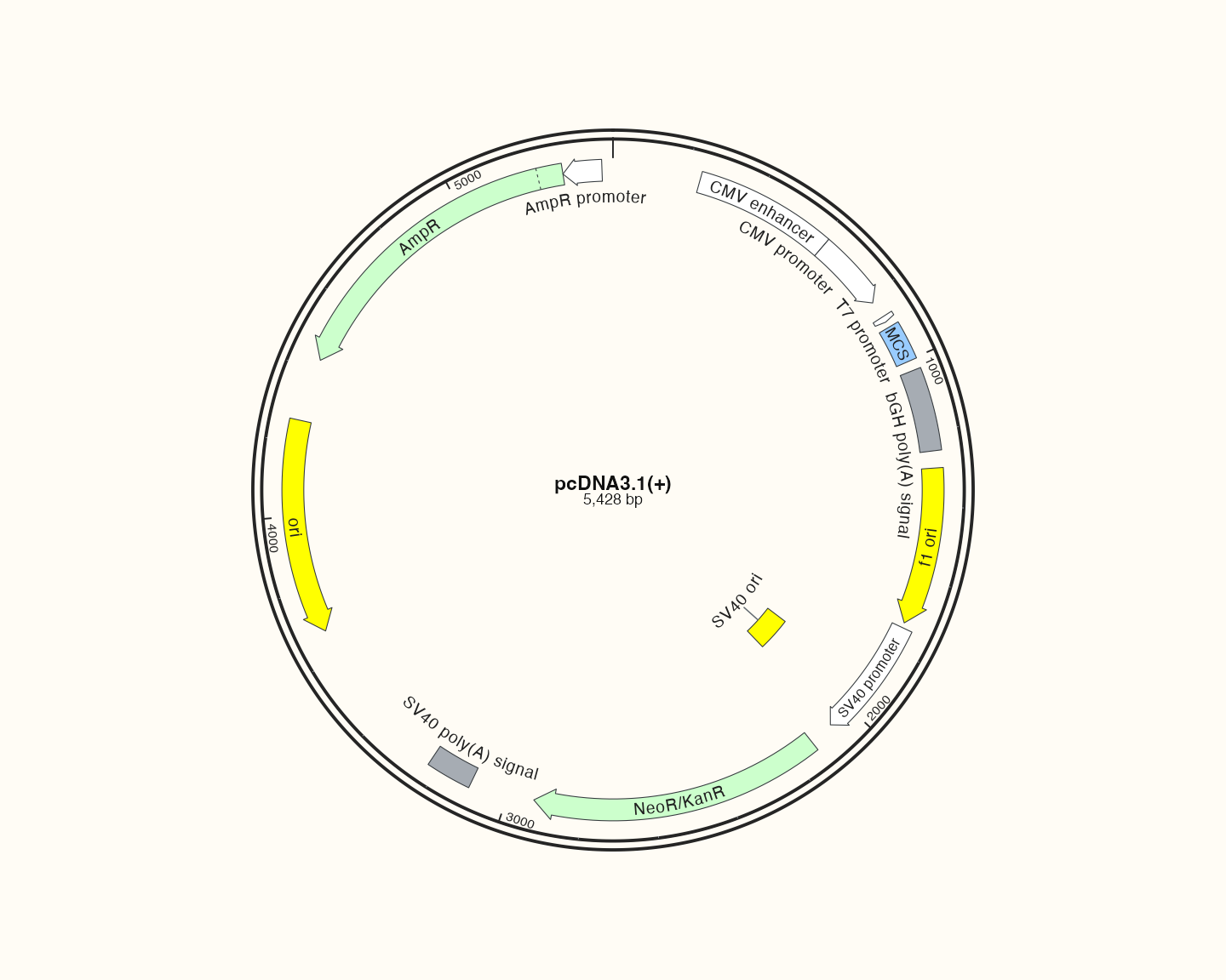
pcDNA3.1(+): Annotation hierarchy in an expression vector
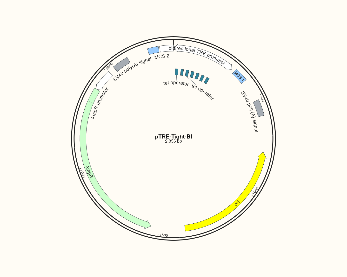
pTRE-Tight-BI: Bidirectional regulatory structure
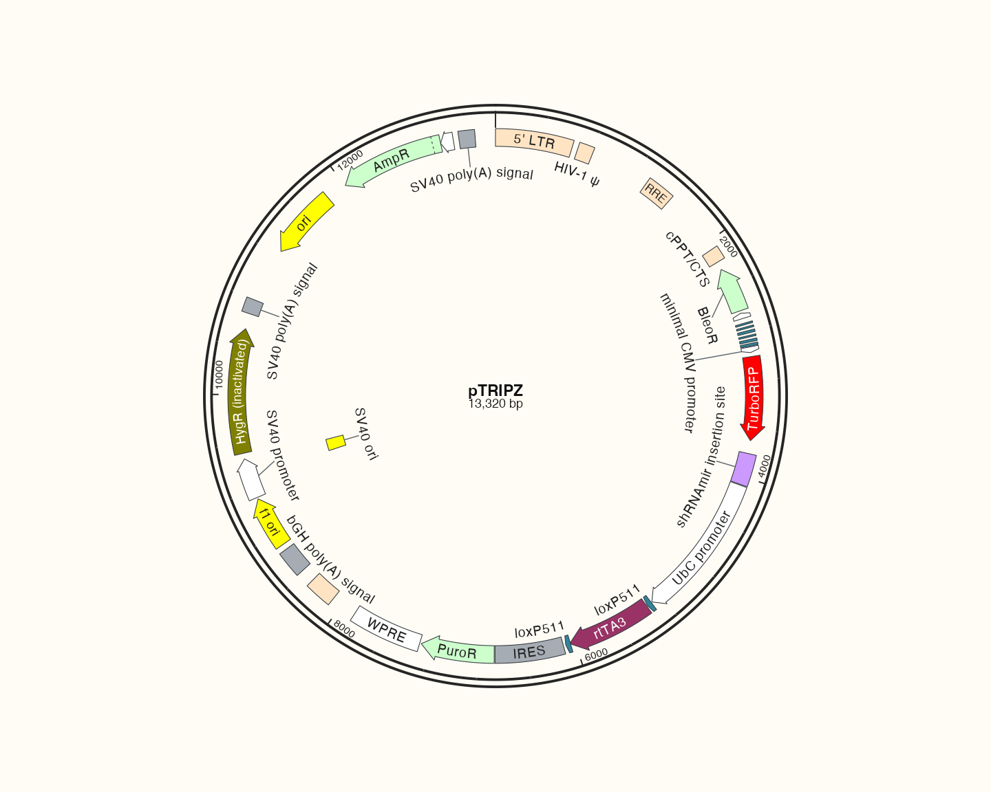
pTRIPZ: Display density on a longer sequence
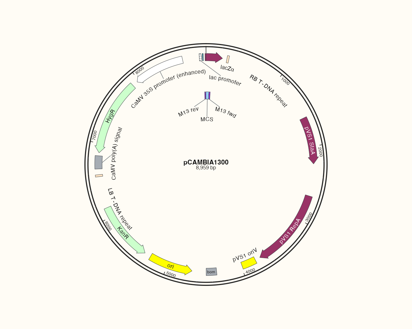
pCAMBIA1300: Architecture of a larger plant vector
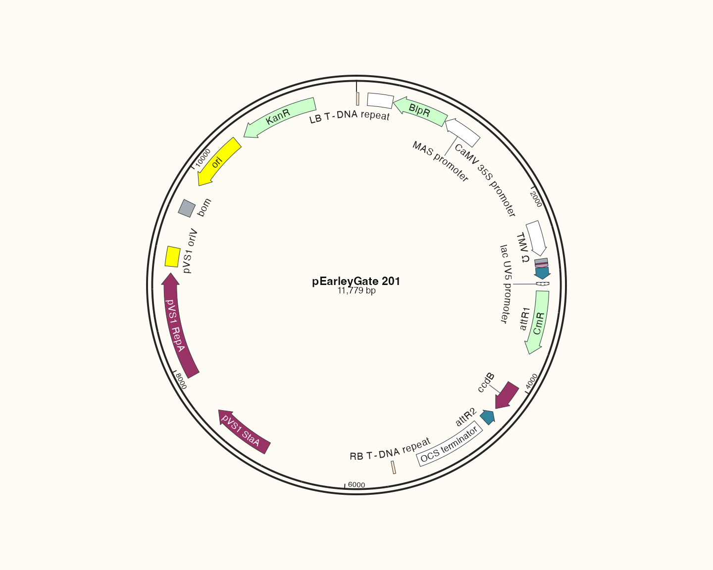
pEarleyGate 201: Category comparison with another plant vector
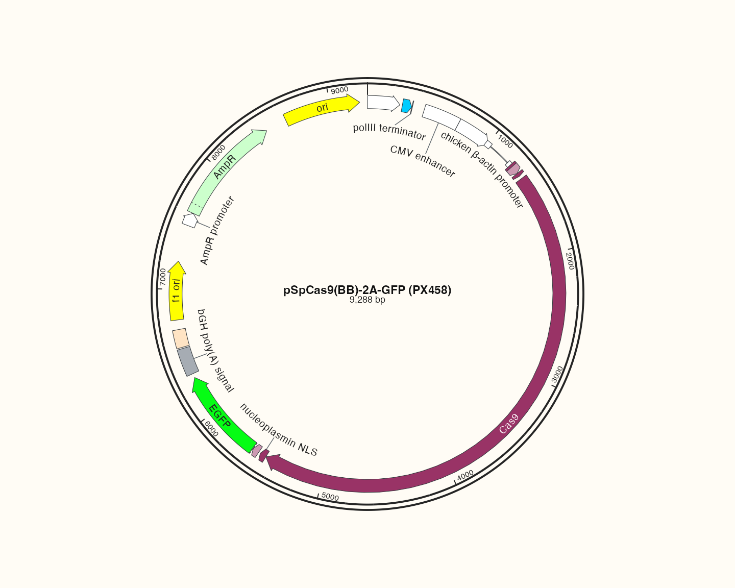
pSpCas9(BB)-2A-GFP (PX458): Large expression vector and label fitting
Next

This gallery contains all 13 unique repository FASTA reference records, redrawn with current code. Historical PNGs and .dna files are not these outputs. Vector roles provide learning prompts rather than experimental validation. Bundled records and their generation rules retain source identity and lengths.

Prepare all cases once

Preparation code — run once on this page

Codelibrary(ggchord)
doc_background <- "#FFFCF5"
identity_palette <- c("#303B71", "#36537D", "#269B82", "#A5D52C", "#ECEB31")
identity_values <- c(0, 0.5, 0.8, 0.9, 1)
identity_breaks <- c(0, 50, 80, 90, 100)
doc_legend_theme <- theme(
  legend.title = element_text(size = 13, face = "bold"),
  legend.text = element_text(size = 11),
  legend.key.width = unit(9, "mm"), legend.key.height = unit(5, "mm"),
  legend.spacing.x = unit(9, "mm"), legend.spacing.y = unit(7, "mm"),
  legend.margin = margin(l = 4, r = 4, unit = "mm")
)
sequence_guide <- guide_ggchord_legend(nrow = 1, theme = doc_legend_theme)
strand_guide <- guide_ggchord_legend(
  nrow = 1, override.aes = list(strand = c("+", "-")), theme = doc_legend_theme
)
identity_guide <- guide_ggchord_colourbar(
  position = "left", direction = "vertical",
  theme = theme(
    legend.key.height = unit(75, "mm"), legend.key.width = unit(5, "mm"),
    legend.title = element_text(size = 13, face = "bold"),
    legend.text = element_text(size = 11), legend.margin = margin(r = 7, unit = "mm")
  )
)
doc_theme <- theme_ggchord_publication(
  axis.text = element_text(size = 11),
  axis.text.check.overlap = TRUE
) +
  theme(
    legend.position = "bottom",
    legend.title = element_text(size = 13, face = "bold"),
    legend.text = element_text(size = 11),
    legend.key.width = unit(9, "mm"), legend.key.height = unit(5, "mm"),
    legend.spacing.x = unit(9, "mm"), legend.spacing.y = unit(7, "mm"),
    legend.box.spacing = unit(6, "mm"),
    plot.background = element_rect(fill = doc_background, colour = NA),
    panel.background = element_blank(),
    plot.title = element_text(face = "bold", size = 18),
    plot.subtitle = element_text(size = 10, colour = "#5C625A"),
    plot.margin = margin(14, 18, 14, 18)
  )
doc_axis <- function(coordinates = "relative") {
  scale_seq_position_continuous(
    coordinates = coordinates, n.breaks = 3, minor_breaks = NULL,
    labels = function(x) format(x, scientific = FALSE, big.mark = ",", trim = TRUE)
  )
}

Codelibrary(ggchord)
library(dplyr)
library(purrr)
# Thirteen unique records; the compatibility spelling pUC19c is not an extra plasmid.
catalog_objects <- c(
  "plasmid_example_pSB1C3", "plasmid_example_pUC19", "plasmid_example_pBR322",
  "plasmid_example_pBluescript_II_SK_plus", "plasmid_example_pET_28a_plus",
  "plasmid_example_pETDuet_1", "plasmid_example_pDONR221",
  "plasmid_example_pcDNA3_1_plus", "plasmid_example_pTRE_Tight_BI",
  "plasmid_example_pTRIPZ", "plasmid_example_pCAMBIA1300",
  "plasmid_example_pEarleyGate_201", "plasmid_example_pSpCas9_BB_2A_GFP_PX458"
)
read_catalog_record <- function(object) {
  target <- new.env(parent = emptyenv())
  data(list = object, package = "ggchord", envir = target)
  target[[object]]
}
catalog_sequences <- map(catalog_objects, read_catalog_record)
catalog_features <- map(catalog_sequences, find_common_features)
catalog_summary <- map2(catalog_sequences, catalog_features, function(sequence, features) {
  tibble(accver = sequence$accver, length = sequence$length, features = nrow(features))
}) |>
  bind_rows()

Codemake_catalog_plot <- function(sequence, features) {
  placement <- position_feature_stack(spacing = 0.085, base_position = position_plasmid())
  ggchord(seq_data = sequence |> select(accver, length)) +
    geom_seq(seq_style = "double", colour = "#252525") +
    geom_feature_plasmid(data = features, position = placement) +
    geom_feature_label_repel(
      data = features, position = placement, external = FALSE,
      label_fit = "shrink", label_min_size = 2.5, max_overlaps = 0
    ) +
    geom_seq_center_label() +
    coord_circular(rotation = 90, fit = "manual", xlim = c(-1.35, 1.35), ylim = c(-1.35, 1.35)) +
    theme_ggchord_plasmid() +
    theme(
      panel.background = element_blank(),
      plot.background = element_rect(fill = doc_background, colour = NA)
    )
}
catalog_plots <- map2(catalog_sequences, catalog_features, make_catalog_plot)
names(catalog_plots) <- catalog_summary$accver
# Save any record at the same size used in the gallery.
# ggsave("pBR322.png", catalog_plots[["pBR322"]], width = 10, height = 8, dpi = 144)

One small function composes independent layers, retaining every recognition result in catalog_features. Actual counts appear below. These maps retain all feature geometry and fit labels inside, allowing labels to hide when space is insufficient; primers and dense restriction annotations are combined in the complete case. Save a named plot with the commented ggsave call.

Inputs and recognition results

Reference	Length (bp)	Features
pSB1C3	2070	7
pUC19	2686	9
pBR322	4361	6
pBluescript II SK(+)	2961	14
pET-28a(+)	5369	16
pETDuet-1	5420	20
pDONR221	4761	11
pcDNA3.1(+)	5428	13
pTRE-Tight-BI	2856	15
pTRIPZ	13320	33
pCAMBIA1300	8959	17
pEarleyGate 201	11779	21
pSpCas9(BB)-2A-GFP (PX458)	9288	19