Chapters and reference
Module I · Multi-sequence relationships · Section 3 of 16
1.2 Four-view comparison and flagship examples
On this page
See Flagship data sources and construction for provenance, display selections and rebuilding. This page loads bundled inputs directly and focuses on plotting settings.
1 Prepare once
The same source input need not produce the same default relation set. First explicitly select all pairs to compare geometry, then inspect each view’s default selection. Dependencies: ggchord and dplyr.
Data preparation and settings (expand)
R · Example code
comparison <- ggchord(radial_seqs, radial_hsp, feature_data = radial_features) +
  geom_seq() +
  geom_seq_label() +
  geom_link_ribbon(adjacent_only = FALSE) +
  geom_feature(shape = "arrow", width = 0.025)
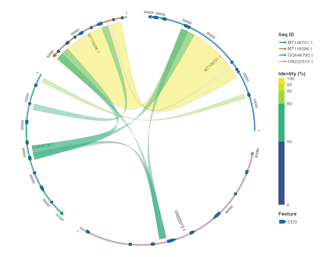
p_coursechord <- comparison + coord_chord()
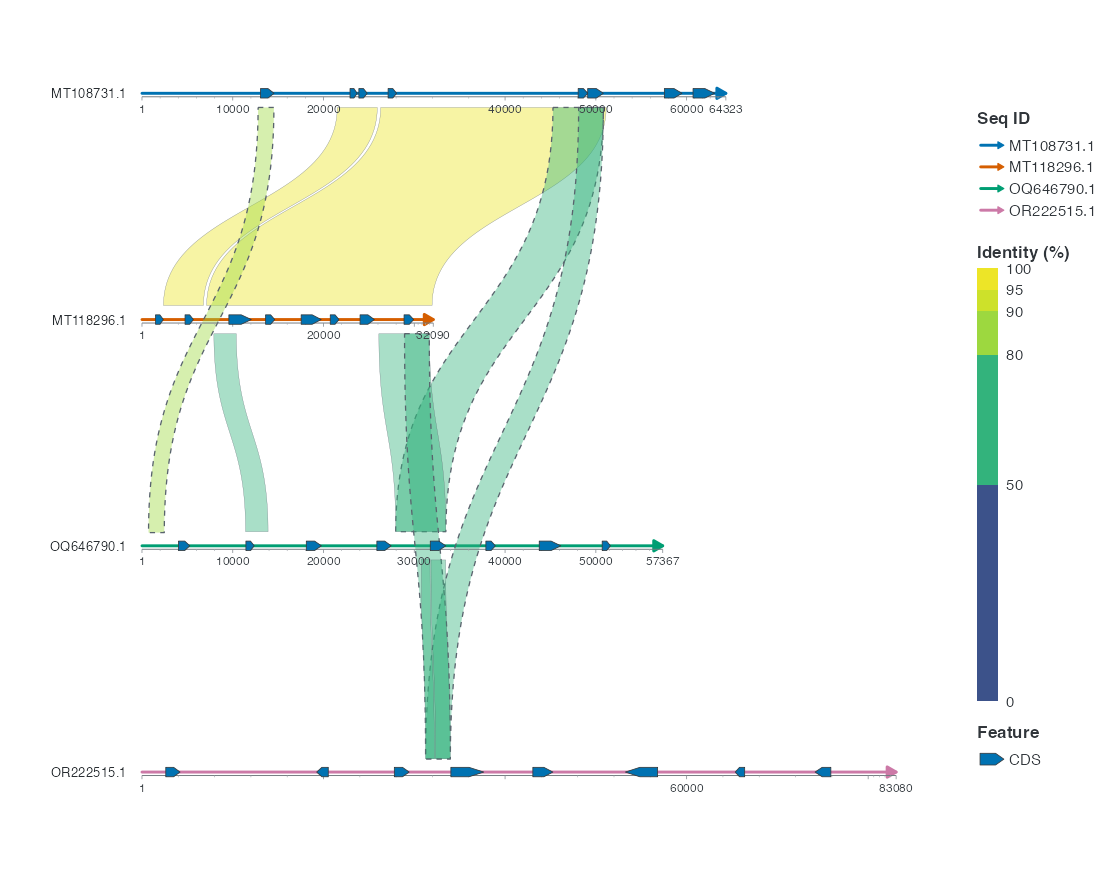
p_courselinear <- comparison + coord_collinear()
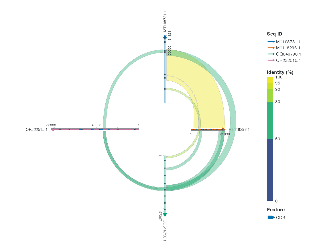
p_courseradial <- comparison + coord_radial_synteny()
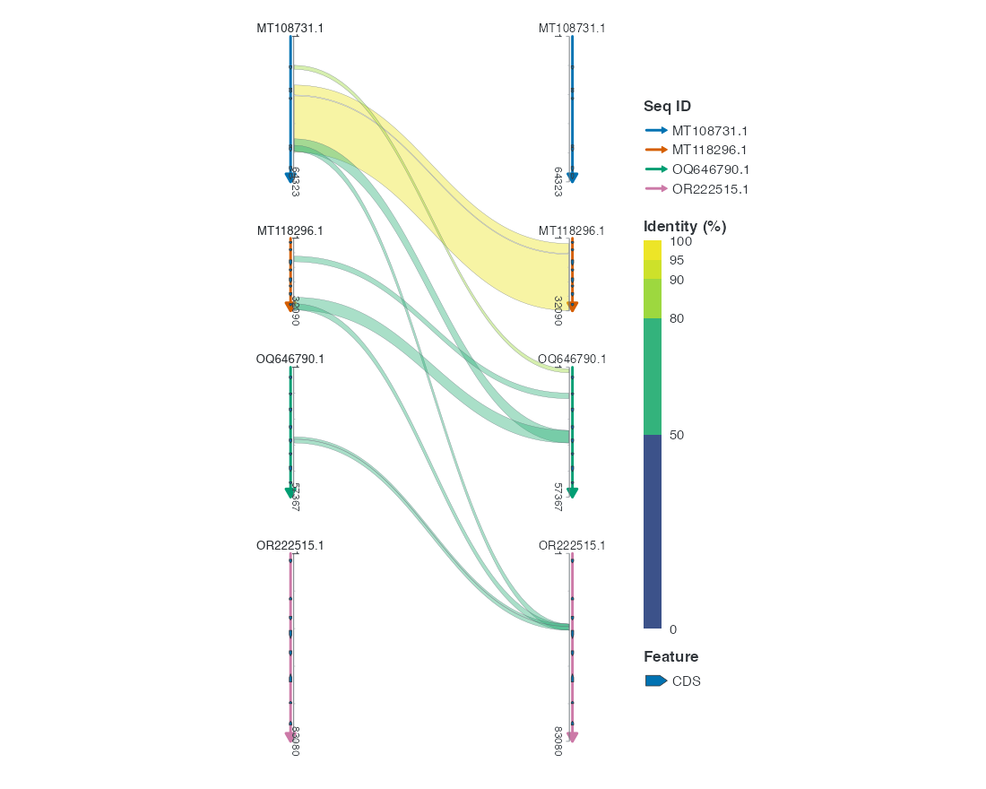
p_coursesankey <- comparison + coord_sankey()
1.1 Chord
1.2 Linear
1.3 Radial
1.4 Sankey
2 Default selection and comparable conditions
| View | Default relation selection | This comparison |
|---|---|---|
| Chord | All pairs | Same HSP table, explicit all pairs |
| Collinear | Adjacent rows | Explicit adjacent_only = FALSE |
| Radial | Cyclic neighbors | Explicit adjacent_only = FALSE |
| Sankey | Excludes same-entity self links | This real input has no self links |
3 Four flagship views
All four views use bundled flagship_comparison_example and run after installing ggchord. Chord/Radial and Collinear/Sankey retain their respective CDS and HSP selections, so their displayed subsets are not identical.
Prepare the shared data, palette and styles once; each view then sets its own geometry, labels and coordinates. The following code requires ggplot2, dplyr and purrr; complete styling is also shown on this page.
R · Example code
# Optional appearance choices; none of these columns or scales is required input.
seq_palette <- setNames(
  c("#E64B35", "#233E4A", "#269B82", "#D59B17"),
  c("MT108731.1", "MT118296.1", "OQ646790.1", "OR222515.1")
)
gene_palette <- c("+" = "#CE1536", "-" = "#346B9D", "." = "#8291A6")

doc_background <- "#FFFCF5"
doc_legend_theme <- theme(
  legend.title = element_text(size = 13, face = "bold"),
  legend.text = element_text(size = 11),
  legend.key.width = unit(9, "mm"), legend.key.height = unit(5, "mm"),
  legend.spacing.x = unit(9, "mm"), legend.spacing.y = unit(7, "mm"),
  legend.margin = margin(l = 4, r = 4, unit = "mm")
)
sequence_guide <- guide_ggchord_legend(nrow = 1, theme = doc_legend_theme)
strand_guide <- guide_ggchord_legend(
  nrow = 1, override.aes = list(strand = c("+", "-")), theme = doc_legend_theme
)
identity_guide_theme <- theme(
  legend.key.height = unit(100, "mm"), legend.key.width = unit(5, "mm"),
  legend.title = element_text(size = 13, face = "bold"),
  legend.text = element_text(size = 11), legend.margin = margin(r = 7, unit = "mm")
)
identity_guide <- ggplot2::guide_coloursteps(
  available_aes = "ribbon_fill", even.steps = FALSE, show.limits = TRUE,
  position = "left", direction = "vertical", theme = identity_guide_theme
)

doc_theme <- theme_ggchord_publication(
  axis.text = element_text(size = 11),
  axis.text.check.overlap = TRUE
) +
  theme(
    legend.position = "bottom",
    legend.title = element_text(size = 13, face = "bold"),
    legend.text = element_text(size = 11),
    legend.key.width = unit(9, "mm"), legend.key.height = unit(5, "mm"),
    legend.spacing.x = unit(9, "mm"), legend.spacing.y = unit(7, "mm"),
    legend.box.spacing = unit(6, "mm"),
    plot.background = element_rect(fill = doc_background, colour = NA),
    panel.background = element_blank(),
    plot.title = element_text(face = "bold", size = 18),
    plot.subtitle = element_text(size = 10, colour = "#5C625A"),
    plot.margin = margin(14, 18, 14, 18)
  )
doc_axis <- function(coordinates = "relative") {
  scale_seq_position_continuous(
    coordinates = coordinates, n.breaks = 3, minor_breaks = NULL,
    labels = function(x) format(x, scientific = FALSE, big.mark = ",", trim = TRUE)
  )
}

library(dplyr)
library(purrr)
data(genome_comparison_example)
show_sequences <- flagship_comparison_example$chord$seq_data
show_annotations <- genome_comparison_example$annotations
show_genes <- genome_comparison_example$genes
show_alignments <- genome_comparison_example$alignments
show_links <- flagship_comparison_example$chord$links
show_features <- genome_comparison_example$features
show_labels <- show_features
show_optimization <- list(seq_orientation = flagship_comparison_example$chord$orientation)

chord_genes <- flagship_comparison_example$chord$features
chord_labels <- flagship_comparison_example$chord$labels
chord_position <- position_strand(c("+" = -0.030, "-" = 0.030))
showcase_style <- list(
  scale_seq_colour_manual(values = seq_palette, name = "Sequence", guide = sequence_guide),
  scale_gene_fill_manual(values = gene_palette, breaks = c("+", "-"), name = "Strand"),
  guides(gene_fill = strand_guide, ribbon_fill = identity_guide),
  doc_axis(), doc_theme
)
Radial removes Chord-only radii and curvature. Sankey uses each column’s native axis, replacing Collinear Cartesian controls and its shared scale bar. Complete figures retain all original CDS name candidates, Sequence guides and source records. Labels are placed near their features in final projected coordinates using measured text sizes and short leaders. Crowded names that cannot fit may still be hidden; use diagnose_ggchord() at the export size to inspect visibility and contacts.
3.1 Chord
R · Example code
show_curvature <- c(
  "MT108731.1" = 0, "MT118296.1" = 1,
  "OQ646790.1" = -0.65, "OR222515.1" = 0.75
)
show_radius <- c(
  "MT108731.1" = 1.08, "MT118296.1" = 0.82,
  "OQ646790.1" = 1.18, "OR222515.1" = 1.02
)
p_show_chord <- ggchord(seq_data = show_sequences, ribbon_data = show_links) +
  geom_link_ribbon(link_avoid = "smooth", alpha = 0.46, linewidth = 0.14) +
  geom_seq(
    seq_orientation = show_optimization$seq_orientation,
    seq_curvature = show_curvature, seq_radius = show_radius,
    seq_gap = 0.06, linewidth = 1.1
  ) +
  geom_gene(data = chord_genes, position = chord_position, width = 0.025) +
  geom_gene_label_repel(
    data = chord_labels, label_layout = "radial", label_wrap = 24,
    size = 2.8, label_max_lines = 3, position = chord_position
  ) +
  geom_seq_label(size = 4, seq_label_radius = 0.77, seq_label_hjust = 0.5) +
  showcase_style +
  coord_chord(rotation = 50) +
  labs(
    title = "Four genomes, one connected view",
    subtitle = "Mixed backbone geometry · CDS sampled by source strand"
  )
view_ggchord(p_show_chord, width = 12, height = 10, units = "in")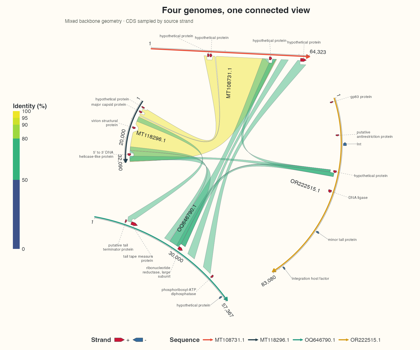
3.2 Collinear
R · Example code
show_linear_features <- flagship_comparison_example$collinear$features
show_adjacent <- flagship_comparison_example$collinear$adjacent_links
show_cross <- flagship_comparison_example$collinear$cross_links
show_linear_coord <- coord_collinear(align = "center", orientation = "auto", ratio = 0.7)
show_cross_controls <- flagship_comparison_example$collinear$route_controls
p_show_collinear <- ggchord(show_sequences, gene_data = show_linear_features) +
  geom_link_ribbon(
    aes(ribbon_fill = pident),
    data = show_adjacent,
    link_avoid = "smooth", alpha = 0.48, linewidth = 0.22
  ) +
  geom_link_ribbon(
    aes(ribbon_fill = pident),
    data = show_cross,
    adjacent_only = FALSE, link_ctrl_point = show_cross_controls,
    link_avoid = "smooth", alpha = 0.28, linewidth = 0.3
  ) +
  geom_seq(seq_gap = 0.42, linewidth = 1) +
  geom_gene(position = position_strand(0.09), width = 0.045) +
  geom_gene_label_repel(
    data = flagship_comparison_example$collinear$labels,
    label_layout = "auto", label_wrap = 24,
    label_side = "auto", position = position_strand(0.09), size = 3.3
  ) +
  geom_seq_label(size = 4) +
  geom_seq_scale(length = 10000, offset = unit(c(0, 10), "mm")) +
  showcase_style +
  show_linear_coord +
  labs(
    title = "Sequence architecture, across four genomes",
    subtitle = "Selected labelled CDS · strand-separated arrows · routed cross-row comparisons"
  )
view_ggchord(p_show_collinear, width = 12, height = 8, units = "in")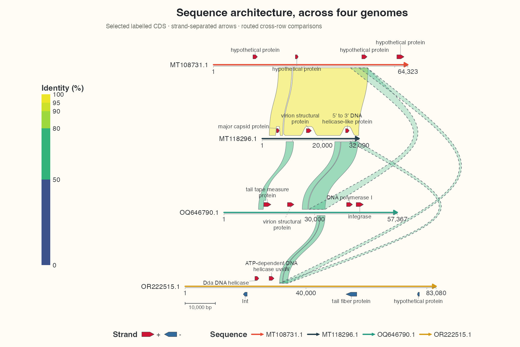
3.3 Radial
R · Example code
relationship_identity <- ggplot2::guide_coloursteps(
  available_aes = "ribbon_fill", even.steps = FALSE, show.limits = TRUE,
  position = "bottom", direction = "horizontal",
  theme = theme(
    legend.key.width = unit(130, "mm"), legend.key.height = unit(4, "mm"),
    legend.title = element_text(size = 10), legend.text = element_text(size = 9),
    legend.margin = margin(2, 2, 2, 2)
  )
)
relationship_guides <- guides(
  seq_colour = guide_ggchord_legend(nrow = 1, position = "bottom"),
  gene_fill = guide_ggchord_legend(
    nrow = 1, position = "bottom", override.aes = list(strand = c("+", "-"))
  ),
  ribbon_fill = relationship_identity
)
relationship_theme <- doc_theme + theme(
  legend.position = "bottom", legend.box = "vertical",
  legend.title = element_text(size = 10, face = "bold"),
  legend.text = element_text(size = 9),
  legend.box.spacing = unit(3, "mm"), legend.spacing.y = unit(2, "mm"),
  legend.margin = margin(2, 2, 2, 2),
  ggchord.axis.text = element_text(size = 9),
  plot.margin = margin(8, 10, 8, 10),
  plot.title = element_text(size = 17), plot.subtitle = element_text(size = 10)
)
relationship_style <- list(
  scale_seq_colour_manual(values = seq_palette, name = "Sequence"),
  scale_gene_fill_manual(values = gene_palette, breaks = c("+", "-"), name = "Strand"),
  scale_seq_position_continuous(n.breaks = 2, minor_breaks = NULL,
    labels = function(x) format(x, scientific = FALSE, big.mark = ",", trim = TRUE)),
  relationship_theme, relationship_guides
)

radial_labels <- flagship_comparison_example$radial$labels
radial_orientation <- flagship_comparison_example$radial$orientation
# Adjustable annular lift for non-neighbours, in layout units; longest spoke = 2.
radial_cross_bulge <- 0.20
radial_position <- position_strand(c("+" = -0.055, "-" = 0.055))
flag_radial <- ggchord(show_sequences, show_links) +
  geom_link_ribbon(adjacent_only = FALSE, link_avoid = "smooth", alpha = 0.46, linewidth = 0.20) +
  geom_seq(seq_orientation = radial_orientation, seq_gap = 0.3, linewidth = 1.1) +
  geom_gene(data = chord_genes, position = radial_position, width = 0.065) +
  geom_gene_label_repel(data = radial_labels, label_side = "auto", label_wrap = 20,
    label_max_lines = 3, position = radial_position, size = 3.1) +
  geom_seq_label(size = 4.4, seq_label_orientation = "horizontal",
    seq_label_vjust = c("MT108731.1" = 0.5, "MT118296.1" = 0.5,
      "OQ646790.1" = 1.5, "OR222515.1" = 0.5)) +
  relationship_style +
  coord_radial_synteny(start_angle = 45, inner_radius = 0.7,
    nonadjacent_bulge = radial_cross_bulge) +
  labs(title = "Four genomes, a radial view", subtitle = "Original Chord sources; all 20 CDS annotations")
Use a 12 × 10.5 inch canvas, spokes starting at 45°, and horizontal sequence IDs. All 20 original CDS geometries and name candidates remain. Local labels avoid long leaders and global side columns that shrink the sequence panel. Sequence, Strand and the numerically proportional Identity guide sit below the plot.
R · Example code
view_ggchord(flag_radial, width = 12, height = 10.5, units = "in")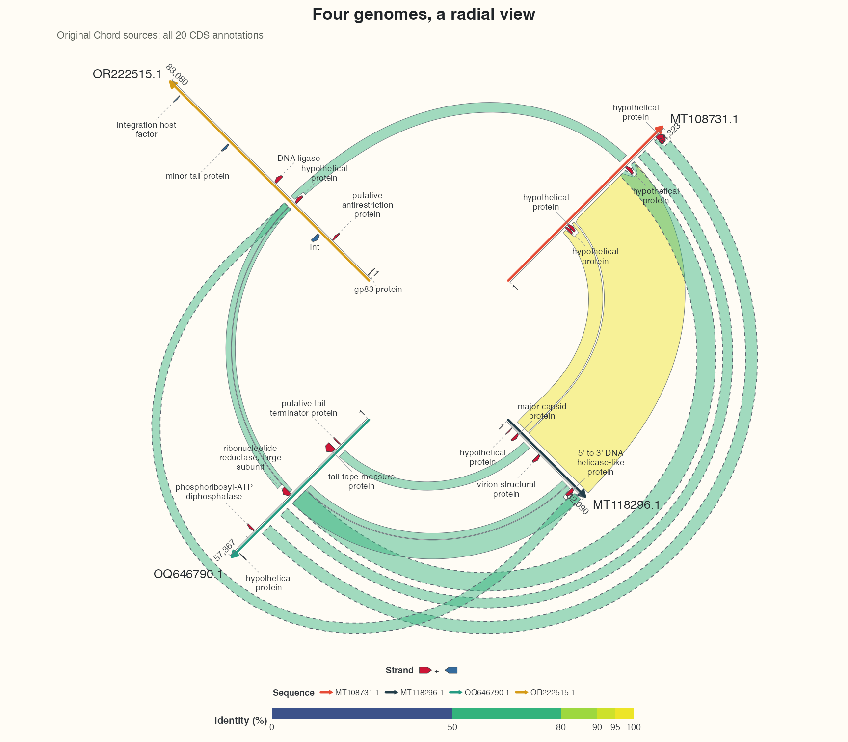
3.4 Sankey
R · Example code
sankey_labels <- flagship_comparison_example$sankey$labels
flag_sankey <- ggchord(show_sequences, gene_data = show_linear_features) +
  geom_link_ribbon(aes(ribbon_fill = pident), data = show_adjacent,
    link_avoid = "smooth", alpha = 0.48, linewidth = 0.25) +
  geom_link_ribbon(aes(ribbon_fill = pident), data = show_cross,
    adjacent_only = FALSE, link_avoid = "smooth", alpha = 0.28, linewidth = 0.3) +
  geom_seq(seq_gap = 0.30, linewidth = 1.1) +
  geom_gene(position = position_strand(0.09), width = 0.075) +
  geom_gene_label_repel(data = sankey_labels, label_wrap = 20,
    label_max_lines = 3, position = position_strand(0.09), size = 3.1) +
  geom_seq_label(size = 4.4) +
  relationship_style +
  coord_sankey(column_gap = 4.2, ratio = 1.15) +
  labs(title = "Four genomes, mirrored relationships", subtitle = "Original Collinear sources; independent query and subject displays")
Four sequences stack in each column on a 10 × 16 inch portrait canvas. All 16 original CDS geometries and name candidates, and the 10 selected HSPs remain. Both display copies receive annotations; names are no longer sampled to one per sequence. Short connections and local collision handling keep names near their features. Complete coordinates and all three guides remain; homepage previews separately omit dense names and coordinate text.
R · Example code
view_ggchord(flag_sankey, width = 10, height = 16, units = "in")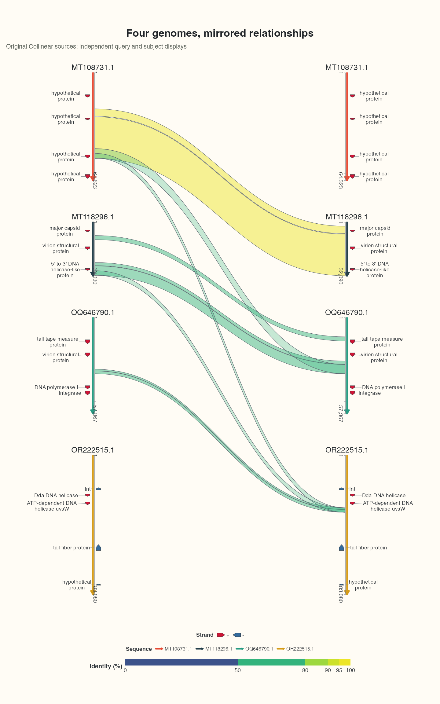
4 Directions, instances and display scale
Biological strand, HSP endpoint direction, display orientation and seq_order are separate. Sankey copies do not add observations; interval widths do not imply flow conservation. Reuse layers only within their shared support.
5 Visual length and connection style
length_mode="equal" changes angular allocation or linear span. Original lengths, intervals and local axes remain unchanged. sequence_display exports both source length and projection factor. A shared absolute scale bar is rejected for equal multi-sequence displays. Default axes show 1 and the final source position; intermediate ticks use available physical space. Closed circular seams combine the two endpoints. Explicit breaks and labels take priority.
Data preparation and settings (expand)
R · Example code
library(dplyr)
foundation_source <- ribbon_data_example |>
  mutate(source_hsp_id = paste0("bundled:", row_number()))
foundation_pair <- foundation_source |>
  slice_head(n = 1) |>
  select(qaccver, saccver)
foundation_ids <- c(foundation_pair$qaccver, foundation_pair$saccver)
foundation_seqs <- seq_data_example |>
  filter(accver %in% foundation_ids) |>
  select(accver, length)
foundation_hsp <- foundation_source |>
  filter(qaccver %in% foundation_ids, saccver %in% foundation_ids,
    qaccver != saccver)
foundation_features <- gene_data_example |>
  filter(accver %in% foundation_ids) |>
  transmute(accver, start, end, strand = source_strand, anno)
R · Example code
p_foundationequal <- ggchord(foundation_seqs, foundation_hsp) +
  geom_seq(length_mode = "equal") +
  geom_link_ribbon(aes(ribbon_fill = pident), tip = "none") +
  coord_collinear()
view_ggchord(p_foundationequal, width = 9, height = 5, units = "in")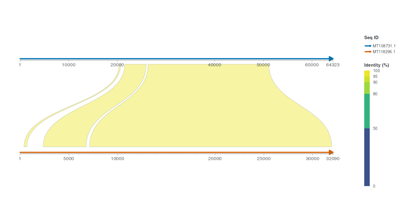
Default ribbons keep Identity fills and full interval fronts. Use geom_link_ribbon(gradient = TRUE) to interpolate endpoint sequence colours along the curve. tip="subject" opts into a decorative taper; its shoulder retains the translated target span and its marker is not a single matched base or a biological transfer direction. The source endpoints stay in layout exports. Use tip="none" to keep full fronts. Fixed fill, mapped ribbon_fill or an explicit ribbon fill scale overrides endpoint interpolation. Explicit pident uses a fixed 0–100 domain, boundaries 0/50/80/90/95/100 and five numerical interval proportions 50/30/10/5/5%. User scales and guides remain authoritative.
5.1 Optional subject taper
R · Example code
p_foundationarrow <- ggchord(foundation_seqs, foundation_hsp) +
  geom_seq() +
  geom_link_ribbon(tip = "subject") +
  coord_collinear()
view_ggchord(p_foundationarrow, width = 9, height = 5, units = "in")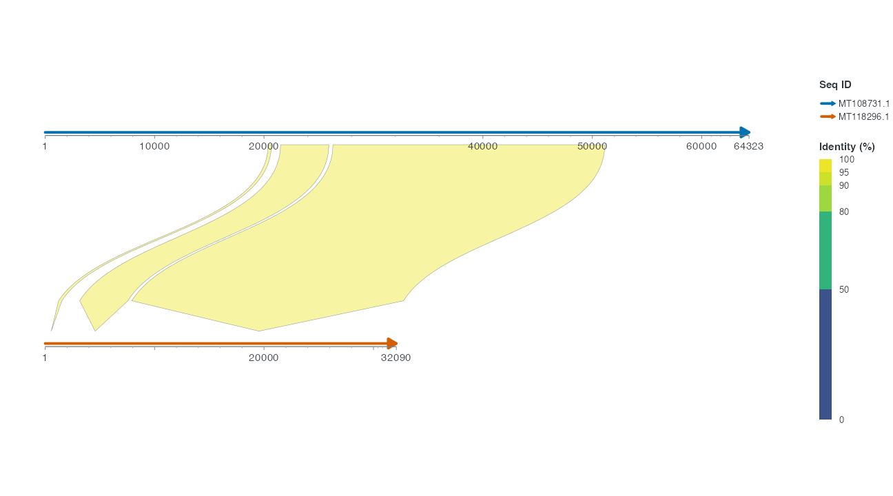
Automatic categorical guides measure text to choose rows/columns, while the render loop measures guide and panel space together. Explicit guide/theme settings win. Circular outer labels share a measured queue at every label count; label_visibility reports source row, visibility and available placement fields. An unavailable collision count is not zero. Tiny canvases can remain crowded; inspect output diagnostics at the intended export size.
Automatic Identity rulers reserve length from measured boundary text rather than generic legend swatch sizes. Set legend.ribbon.key.height or legend.ribbon.key.width, or supply an explicit guide, for a manual length. In circular layouts, parallel axis labels follow the circle glyph by glyph; horizontal and numeric orientations remain straight.
6 Preview and save
Choose an HSP and identify its two sources. Restore default adjacency and explain a possible omission. Save your chosen view at target size and retain the input table.