0.16.6 documentation

Site guide · find your task

Setup and learning paths

HomeInstall and prepare the environmentChoose your learning module

Module I · Chord

1.1 Tables and field meanings1.2 Produce and import comparisons1.3 Build the layers step by step1.4 Direction, curvature and clearance1.5 Filter and summarize links1.6 Full source-file workflow1.7 Complete chord showcase

Module II · Collinear

2.1 Reuse chord input tables2.2 Switch coordinates and add layers2.3 Routes, clearance and the ruler2.4 Compare CDS neighbourhoods2.5 Focus, anchors and segments2.6 Complete collinear showcase

Module III · Plasmid

3.1 DNA, annotations and 13 references3.2 From a circle to annotation layers3.3 Features, primers and restriction3.4 Thirteen plasmid references3.5 Complete plasmid cases

Consult as needed · Data and layers

Prepare tables and coordinatesImport and convert dataImport nucleotide and protein alignmentsProject protein intervals to genomic coordinatesFeatures, stacking and genomic decorationLabels and local placementQuantitative tracksMappings, scales, guides and themesSet values by sequence and strandCommon adjustments and grammarExport, preview and diagnostics

Learning map and reference

Articles and complete workflowsFunction referenceReproducible galleryFrequently asked questionsMigrate to the candidate APITerminology and design sourcesDevelopment status and changes

Install and prepare the environment

On this page

• Install and inspect the environment
• Which version are you using?
• Support evidence
• Choose a learning path
• Which columns come first?
• Optional: check one complete plot
• Read the quick result
• Optional: save the quick result
• Common execution problems

Install and confirm the environment, then choose one progressive module. Reading the entire reference is not a prerequisite.

Install and inspect the environment

R ≥4.1.0 and ggplot2 ≥4.0.0 are required. Installation and examples target v0.16.6.

Code

install.packages(c("remotes", "dplyr", "purrr", "tidyr"))
remotes::install_github("DangJem/ggchord@v0.16.6")
library(ggchord)
packageVersion("ggchord")

Which version are you using?

This tutorial documents ggchord 0.16.6. The installation above pins its formal tag; see GitHub Releases for release assets. For a source checkout, run from its repository root:

Code

install.packages("pkgload")
pkgload::load_all(".")
packageVersion("ggchord")

Use the loading route appropriate to your source; you do not need both installation paths. Record the version when reproducing a plot. This lesson needs neither optional Bioconductor packages nor Biopython.

Support evidence

Declared lower bounds are R 4.1.0 and ggplot2 4.0.0. Release checks and actual platform versions are recorded in the release acceptance report; these do not certify every dependency combination. Optional readers require their documented dependencies.

Choose a learning path

1. Module I · Chord: learn the three tables, then import, backbones, layers and geometry.
2. Module II · Collinear: reuse the chord inputs, then switch coordinates, route links and focus locally.
3. Module III · Plasmid: start with one sequence and DNA, then add layers and explore 13 reference cases.

Starting with chord follows ggchord’s development order. See the learning map. The two-sequence exercise below is an optional environment check rather than a substitute for the modules.

Which columns come first?

Sequences need accver/length; links need two IDs and four endpoints; genes need accver/start/end/strand. Module I’s first lesson explains real tables, optional fields and BLAST naming.

Optional: check one complete plot

Run the whole folded block, then inspect the figure. Bundled source-backed records need no external files or BLAST run.

Preparation code — run once on this page

Code

library(ggchord)
library(dplyr)
data(seq_data_example)
data(gene_data_example)
data(ribbon_data_example)
ids <- c("MT108731.1", "MT118296.1")
first_sequences <- seq_data_example |>
  filter(accver %in% ids) |>
  select(accver, length)
first_genes <- gene_data_example |>
  filter(accver %in% ids) |>
  transmute(accver, start, end, strand = source_strand)
first_links <- ribbon_data_example |>
  filter(qaccver %in% ids, saccver %in% ids) |>
  select(qaccver, saccver, qstart, qend, sstart, send)

first_colours <- setNames(c("#E64B35", "#233E4A"), ids)
p_first <- ggchord(
  seq_data = first_sequences, ribbon_data = first_links,
  gene_data = first_genes
) +
  geom_link_ribbon(fill = "#82B6AD", alpha = .55) +
  geom_seq(colour = "#233E4A", show.legend = FALSE) +
  geom_gene(aes(gene_fill = accver), position = position_strand(.10), width = .045) +
  geom_seq_label(size = 4) +
  coord_collinear() +
  scale_gene_fill_manual(
    values = first_colours, name = "Sequence",
    guide = guide_ggchord_legend(nrow = 1, theme = theme(
      legend.title = element_text(size = 13, face = "bold"), legend.text = element_text(size = 11),
      legend.key.width = unit(9, "mm"), legend.key.height = unit(5, "mm"), legend.margin = margin(l = 7, unit = "mm")
    ))
  ) +
  scale_seq_position_continuous(n.breaks = 3, minor_breaks = NULL) +
  theme_ggchord_publication(axis.text = element_text(size = 11)) +
  theme(
    legend.position = "bottom",
    plot.background = element_rect(fill = "#FFFCF5", colour = NA),
    panel.background = element_blank()
  )
p_first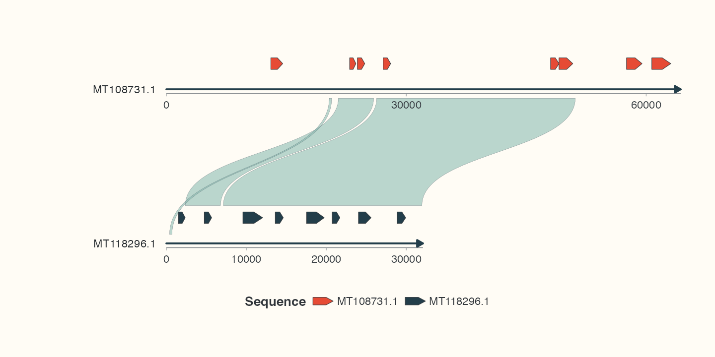

Your first plot: two bundled sequences, gene arrows and observed alignment intervals · Click to enlarge

Read the quick result

Arrows retain biological strands; colours identify sequences only. Ribbons are existing comparison intervals, not new homology results. This small linear example makes positions easy to read; the full chord module starts with backbones.

Optional: save the quick result

Run this only after the block above has created p_first:

Code

ggsave("first-comparison.png", p_first, width = 10, height = 5, units = "in", dpi = 144)

Use the same 10×5 in dimensions for preview and export; see output.

Common execution problems

For missing objects, run the preparation block. For missing functions, check the package version. getwd() determines the save directory. Optional readers need dependencies only in their own topics; basic modules do not require Bioconductor or Biopython.