章节与参考
模块一 · 多序列关系 · 第 3 节,共 16 节
1.2 四视图对照与旗舰实例
本页目录
数据来源、展示子集与重建规则见旗舰数据来源与构建。本页直接加载随包输入,集中设置绘图参数。
1 一次准备
相同来源输入不代表默认展示完全相同的关系。本例先明确全对选择再比较几何;随后核对各视图默认筛选。依赖:ggchord、dplyr。
准备数据与配置(展开)
R · 示例代码
comparison <- ggchord(radial_seqs, radial_hsp, feature_data = radial_features) +
  geom_seq() +
  geom_seq_label() +
  geom_link_ribbon(adjacent_only = FALSE) +
  geom_feature(shape = "arrow", width = 0.025)
p_coursechord <- comparison + coord_chord()
p_courselinear <- comparison + coord_collinear()
p_courseradial <- comparison + coord_radial_synteny()
p_coursesankey <- comparison + coord_sankey()
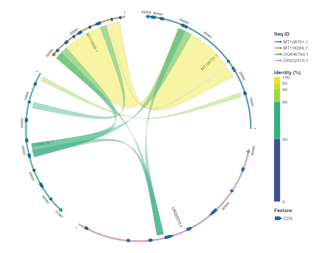
1.1 Chord
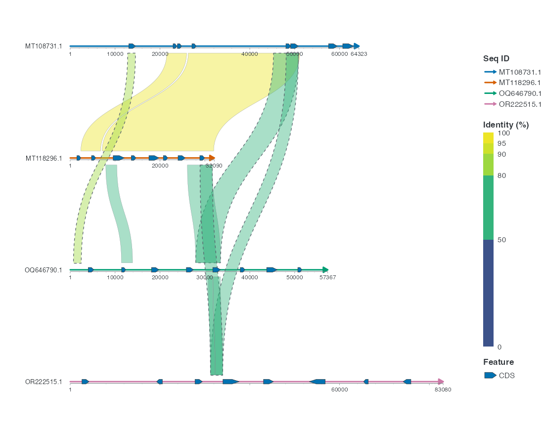
1.2 Linear
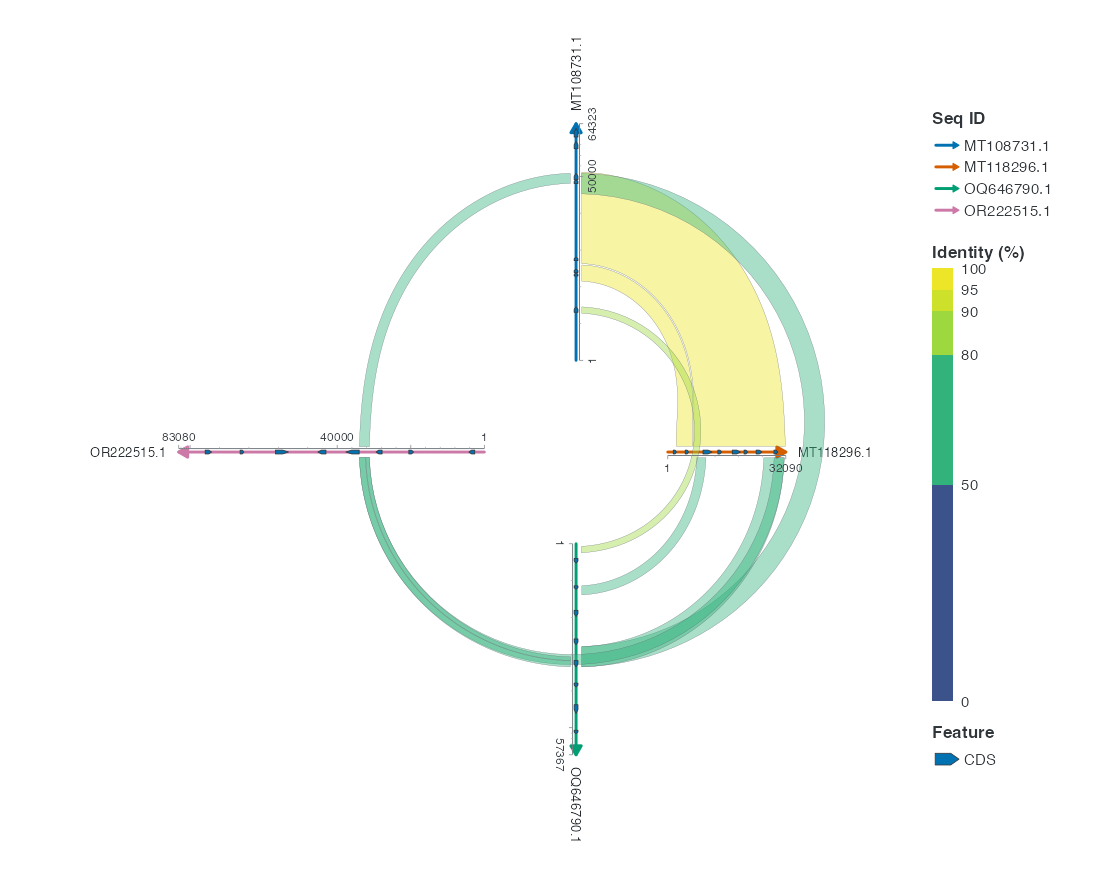
1.3 Radial
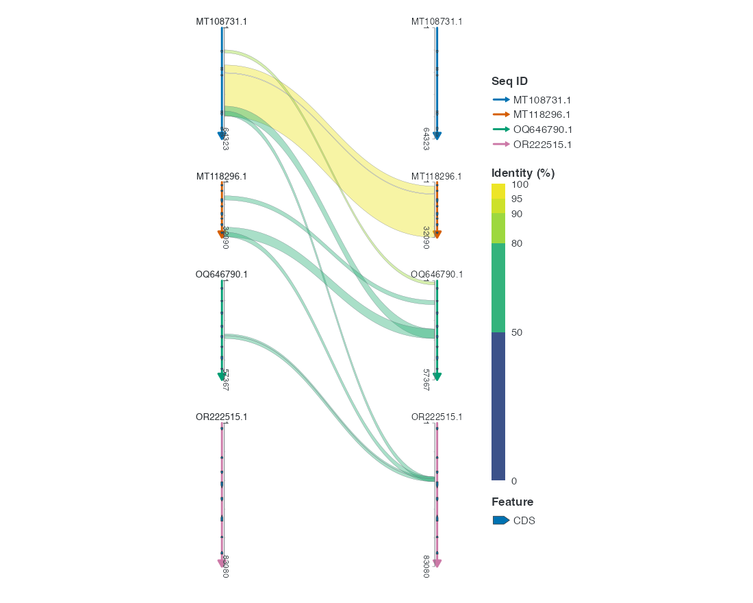
1.4 Sankey
2 默认选择与可比条件
| 视图 | 默认关系选择 | 本例条件 |
|---|---|---|
| Chord | 全对 | 同一 HSP 表,显式全对 |
| Collinear | 相邻行 | 显式 adjacent_only = FALSE |
| Radial | 环形邻居 | 显式 adjacent_only = FALSE |
| Sankey | 排除同实体自身关系 | 本例真实表不含自身关系 |
3 四种旗舰视图
四图共用随包数据 flagship_comparison_example,安装 ggchord 后即可运行。Chord/Radial 与 Collinear/Sankey 保留各自的 CDS 和 HSP 选择,不能视为完全相同的显示子集。
先准备共用数据、配色和样式;各图只设置自己的几何、标签和坐标参数。以下需要 ggplot2、dplyr 和 purrr;完整样式也在本页列出。
R · 示例代码
# 以下为可选外观设置。
seq_palette <- setNames(
  c("#E64B35", "#233E4A", "#269B82", "#D59B17"),
  c("MT108731.1", "MT118296.1", "OQ646790.1", "OR222515.1")
)
gene_palette <- c("+" = "#CE1536", "-" = "#346B9D", "." = "#8291A6")

doc_background <- "#FFFCF5"
doc_legend_theme <- theme(
  legend.title = element_text(size = 13, face = "bold"),
  legend.text = element_text(size = 11),
  legend.key.width = unit(9, "mm"), legend.key.height = unit(5, "mm"),
  legend.spacing.x = unit(9, "mm"), legend.spacing.y = unit(7, "mm"),
  legend.margin = margin(l = 4, r = 4, unit = "mm")
)
sequence_guide <- guide_ggchord_legend(nrow = 1, theme = doc_legend_theme)
strand_guide <- guide_ggchord_legend(
  nrow = 1, override.aes = list(strand = c("+", "-")), theme = doc_legend_theme
)
identity_guide_theme <- theme(
  legend.key.height = unit(100, "mm"), legend.key.width = unit(5, "mm"),
  legend.title = element_text(size = 13, face = "bold"),
  legend.text = element_text(size = 11), legend.margin = margin(r = 7, unit = "mm")
)
identity_guide <- ggplot2::guide_coloursteps(
  available_aes = "ribbon_fill", even.steps = FALSE, show.limits = TRUE,
  position = "left", direction = "vertical", theme = identity_guide_theme
)

doc_theme <- theme_ggchord_publication(
  axis.text = element_text(size = 11),
  axis.text.check.overlap = TRUE
) +
  theme(
    legend.position = "bottom",
    legend.title = element_text(size = 13, face = "bold"),
    legend.text = element_text(size = 11),
    legend.key.width = unit(9, "mm"), legend.key.height = unit(5, "mm"),
    legend.spacing.x = unit(9, "mm"), legend.spacing.y = unit(7, "mm"),
    legend.box.spacing = unit(6, "mm"),
    plot.background = element_rect(fill = doc_background, colour = NA),
    panel.background = element_blank(),
    plot.title = element_text(face = "bold", size = 18),
    plot.subtitle = element_text(size = 10, colour = "#5C625A"),
    plot.margin = margin(14, 18, 14, 18)
  )
doc_axis <- function(coordinates = "relative") {
  scale_seq_position_continuous(
    coordinates = coordinates, n.breaks = 3, minor_breaks = NULL,
    labels = function(x) format(x, scientific = FALSE, big.mark = ",", trim = TRUE)
  )
}

library(dplyr)
library(purrr)
data(genome_comparison_example)
show_sequences <- flagship_comparison_example$chord$seq_data
show_annotations <- genome_comparison_example$annotations
show_genes <- genome_comparison_example$genes
show_alignments <- genome_comparison_example$alignments
show_links <- flagship_comparison_example$chord$links
show_features <- genome_comparison_example$features
show_labels <- show_features
show_optimization <- list(seq_orientation = flagship_comparison_example$chord$orientation)

chord_genes <- flagship_comparison_example$chord$features
chord_labels <- flagship_comparison_example$chord$labels
chord_position <- position_strand(c("+" = -0.030, "-" = 0.030))
showcase_style <- list(
  scale_seq_colour_manual(values = seq_palette, name = "Sequence", guide = sequence_guide),
  scale_gene_fill_manual(values = gene_palette, breaks = c("+", "-"), name = "Strand"),
  guides(gene_fill = strand_guide, ribbon_fill = identity_guide),
  doc_axis(), doc_theme
)
Radial 移除 Chord 专属的半径和曲率;Sankey 使用各列原生坐标轴,不照搬 Collinear 的 Cartesian 控制点和共享比例尺。完整图保留所有原 CDS 名称候选、序列图例和来源记录。注释在最终投影坐标中按真实文字尺寸避让,优先邻近特征的短引导线;数据密集时仍可能隐藏无法安放的名称,可用 diagnose_ggchord() 查看实际导出尺寸下的显示与碰撞结果。
3.1 Chord
R · 示例代码
show_curvature <- c(
  "MT108731.1" = 0, "MT118296.1" = 1,
  "OQ646790.1" = -0.65, "OR222515.1" = 0.75
)
show_radius <- c(
  "MT108731.1" = 1.08, "MT118296.1" = 0.82,
  "OQ646790.1" = 1.18, "OR222515.1" = 1.02
)
p_show_chord <- ggchord(seq_data = show_sequences, ribbon_data = show_links) +
  geom_link_ribbon(link_avoid = "smooth", alpha = 0.46, linewidth = 0.14) +
  geom_seq(
    seq_orientation = show_optimization$seq_orientation,
    seq_curvature = show_curvature, seq_radius = show_radius,
    seq_gap = 0.06, linewidth = 1.1
  ) +
  geom_gene(data = chord_genes, position = chord_position, width = 0.025) +
  geom_gene_label_repel(
    data = chord_labels, label_layout = "radial", label_wrap = 24,
    size = 2.8, label_max_lines = 3, position = chord_position
  ) +
  geom_seq_label(size = 4, seq_label_radius = 0.77, seq_label_hjust = 0.5) +
  showcase_style +
  coord_chord(rotation = 50) +
  labs(
    title = "Four genomes, one connected view",
    subtitle = "Mixed backbone geometry · CDS sampled by source strand"
  )
view_ggchord(p_show_chord, width = 12, height = 10, units = "in")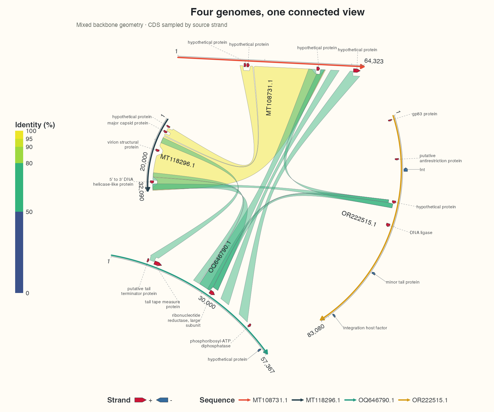
3.2 Collinear
R · 示例代码
show_linear_features <- flagship_comparison_example$collinear$features
show_adjacent <- flagship_comparison_example$collinear$adjacent_links
show_cross <- flagship_comparison_example$collinear$cross_links
show_linear_coord <- coord_collinear(align = "center", orientation = "auto", ratio = 0.7)
show_cross_controls <- flagship_comparison_example$collinear$route_controls
p_show_collinear <- ggchord(show_sequences, gene_data = show_linear_features) +
  geom_link_ribbon(
    aes(ribbon_fill = pident),
    data = show_adjacent,
    link_avoid = "smooth", alpha = 0.48, linewidth = 0.22
  ) +
  geom_link_ribbon(
    aes(ribbon_fill = pident),
    data = show_cross,
    adjacent_only = FALSE, link_ctrl_point = show_cross_controls,
    link_avoid = "smooth", alpha = 0.28, linewidth = 0.3
  ) +
  geom_seq(seq_gap = 0.42, linewidth = 1) +
  geom_gene(position = position_strand(0.09), width = 0.045) +
  geom_gene_label_repel(
    data = flagship_comparison_example$collinear$labels,
    label_layout = "auto", label_wrap = 24,
    label_side = "auto", position = position_strand(0.09), size = 3.3
  ) +
  geom_seq_label(size = 4) +
  geom_seq_scale(length = 10000, offset = unit(c(0, 10), "mm")) +
  showcase_style +
  show_linear_coord +
  labs(
    title = "Sequence architecture, across four genomes",
    subtitle = "Selected labelled CDS · strand-separated arrows · routed cross-row comparisons"
  )
view_ggchord(p_show_collinear, width = 12, height = 8, units = "in")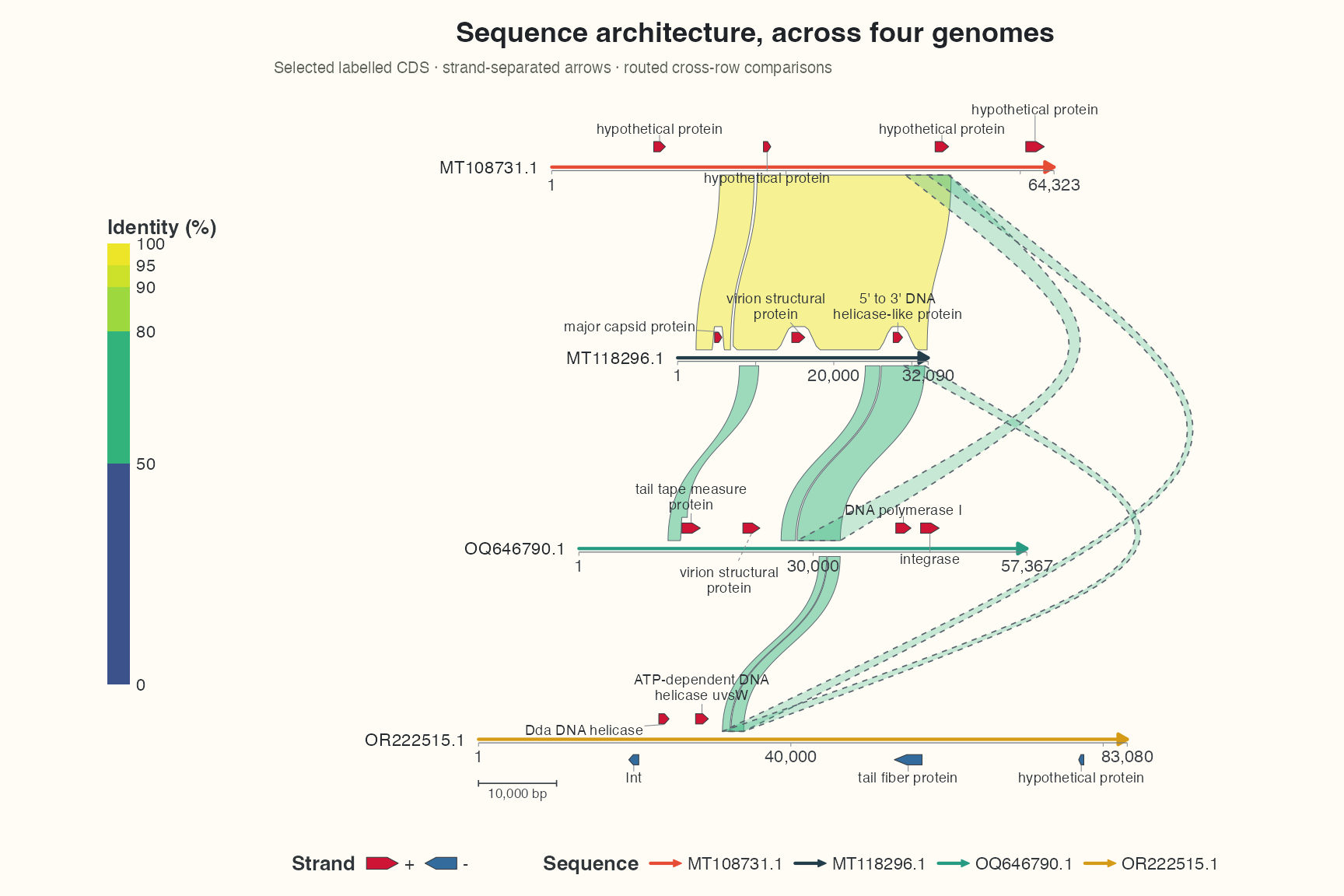
3.3 Radial
R · 示例代码
relationship_identity <- ggplot2::guide_coloursteps(
  available_aes = "ribbon_fill", even.steps = FALSE, show.limits = TRUE,
  position = "bottom", direction = "horizontal",
  theme = theme(
    legend.key.width = unit(130, "mm"), legend.key.height = unit(4, "mm"),
    legend.title = element_text(size = 10), legend.text = element_text(size = 9),
    legend.margin = margin(2, 2, 2, 2)
  )
)
relationship_guides <- guides(
  seq_colour = guide_ggchord_legend(nrow = 1, position = "bottom"),
  gene_fill = guide_ggchord_legend(
    nrow = 1, position = "bottom", override.aes = list(strand = c("+", "-"))
  ),
  ribbon_fill = relationship_identity
)
relationship_theme <- doc_theme + theme(
  legend.position = "bottom", legend.box = "vertical",
  legend.title = element_text(size = 10, face = "bold"),
  legend.text = element_text(size = 9),
  legend.box.spacing = unit(3, "mm"), legend.spacing.y = unit(2, "mm"),
  legend.margin = margin(2, 2, 2, 2),
  ggchord.axis.text = element_text(size = 9),
  plot.margin = margin(8, 10, 8, 10),
  plot.title = element_text(size = 17), plot.subtitle = element_text(size = 10)
)
relationship_style <- list(
  scale_seq_colour_manual(values = seq_palette, name = "Sequence"),
  scale_gene_fill_manual(values = gene_palette, breaks = c("+", "-"), name = "Strand"),
  scale_seq_position_continuous(n.breaks = 2, minor_breaks = NULL,
    labels = function(x) format(x, scientific = FALSE, big.mark = ",", trim = TRUE)),
  relationship_theme, relationship_guides
)

radial_labels <- flagship_comparison_example$radial$labels
radial_orientation <- flagship_comparison_example$radial$orientation
# 可调整非相邻环形连接的外拱量,单位为布局单位;最长辐条为2。
radial_cross_bulge <- 0.20
radial_position <- position_strand(c("+" = -0.055, "-" = 0.055))
flag_radial <- ggchord(show_sequences, show_links) +
  geom_link_ribbon(adjacent_only = FALSE, link_avoid = "smooth", alpha = 0.46, linewidth = 0.20) +
  geom_seq(seq_orientation = radial_orientation, seq_gap = 0.3, linewidth = 1.1) +
  geom_gene(data = chord_genes, position = radial_position, width = 0.065) +
  geom_gene_label_repel(data = radial_labels, label_side = "auto", label_wrap = 20,
    label_max_lines = 3, position = radial_position, size = 3.1) +
  geom_seq_label(size = 4.4, seq_label_orientation = "horizontal",
    seq_label_vjust = c("MT108731.1" = 0.5, "MT118296.1" = 0.5,
      "OQ646790.1" = 1.5, "OR222515.1" = 0.5)) +
  relationship_style +
  coord_radial_synteny(start_angle = 45, inner_radius = 0.7,
    nonadjacent_bulge = radial_cross_bulge) +
  labs(title = "Four genomes, a radial view", subtitle = "Original Chord sources; all 20 CDS annotations")
采用 12 × 10.5 英寸画布,辐条从 45° 起排、序列名水平显示。保留全部 20 条原 CDS 几何与名称候选,名称随源特征就近安排,避免全局两侧名列和长引导线压缩序列主体。Sequence、Strand 与按数值区间比例显示的 Identity 图例集中在下方。
R · 示例代码
view_ggchord(flag_radial, width = 12, height = 10.5, units = "in")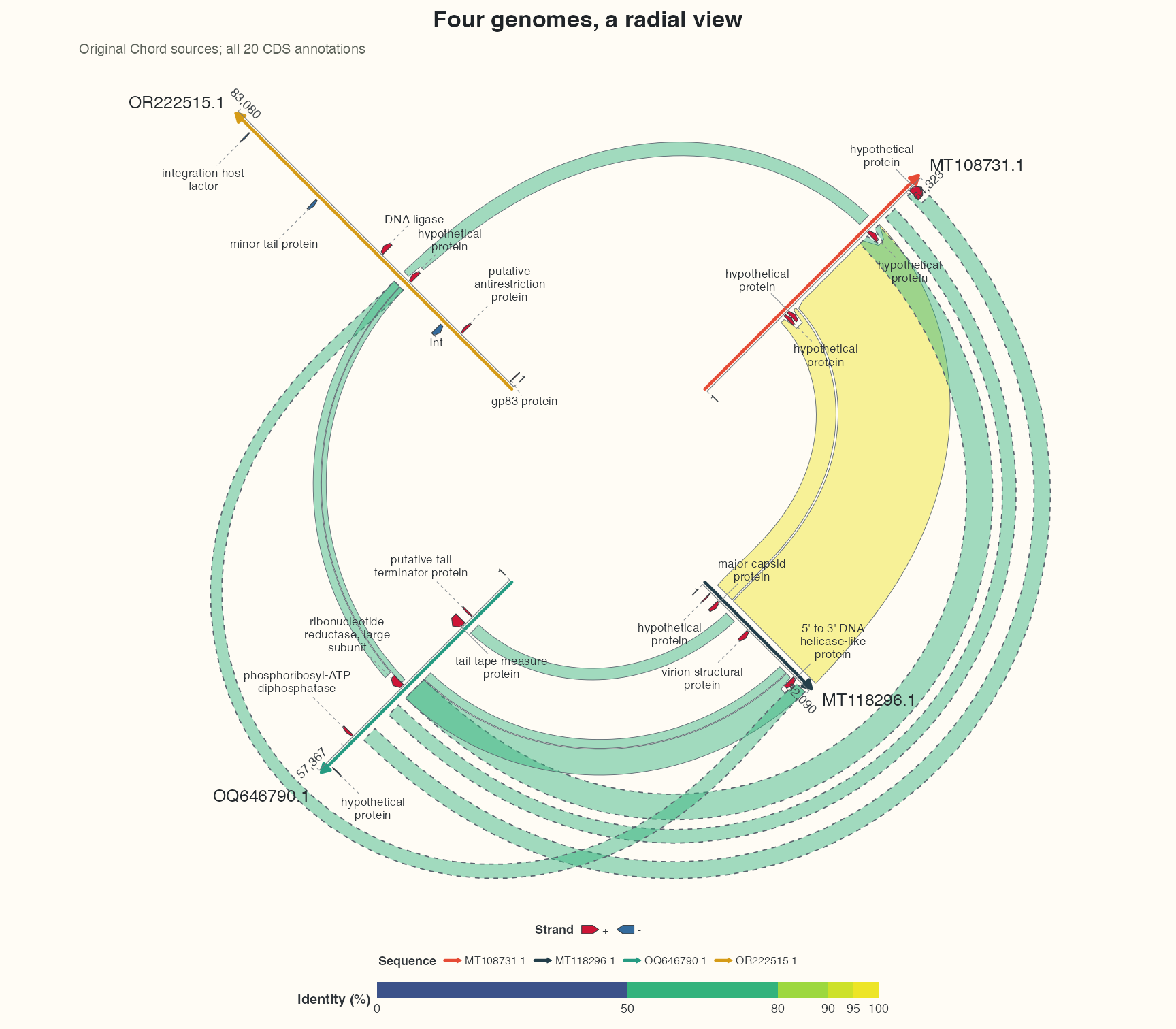
3.4 Sankey
R · 示例代码
sankey_labels <- flagship_comparison_example$sankey$labels
flag_sankey <- ggchord(show_sequences, gene_data = show_linear_features) +
  geom_link_ribbon(aes(ribbon_fill = pident), data = show_adjacent,
    link_avoid = "smooth", alpha = 0.48, linewidth = 0.25) +
  geom_link_ribbon(aes(ribbon_fill = pident), data = show_cross,
    adjacent_only = FALSE, link_avoid = "smooth", alpha = 0.28, linewidth = 0.3) +
  geom_seq(seq_gap = 0.30, linewidth = 1.1) +
  geom_gene(position = position_strand(0.09), width = 0.075) +
  geom_gene_label_repel(data = sankey_labels, label_wrap = 20,
    label_max_lines = 3, position = position_strand(0.09), size = 3.1) +
  geom_seq_label(size = 4.4) +
  relationship_style +
  coord_sankey(column_gap = 4.2, ratio = 1.15) +
  labs(title = "Four genomes, mirrored relationships", subtitle = "Original Collinear sources; independent query and subject displays")
四条序列在两列中纵向排列,使用 10 × 16 英寸纵向画布。16 条原 CDS 几何与名称候选、10 条已选择 HSP 均保留;左右副本分别标注,名称不再每序列只选一条。列外的短连接与局部避让保持文字靠近对应特征;完整刻度和三组图例保留。首页预览另省略密集名称和坐标文字。
R · 示例代码
view_ggchord(flag_sankey, width = 10, height = 16, units = "in")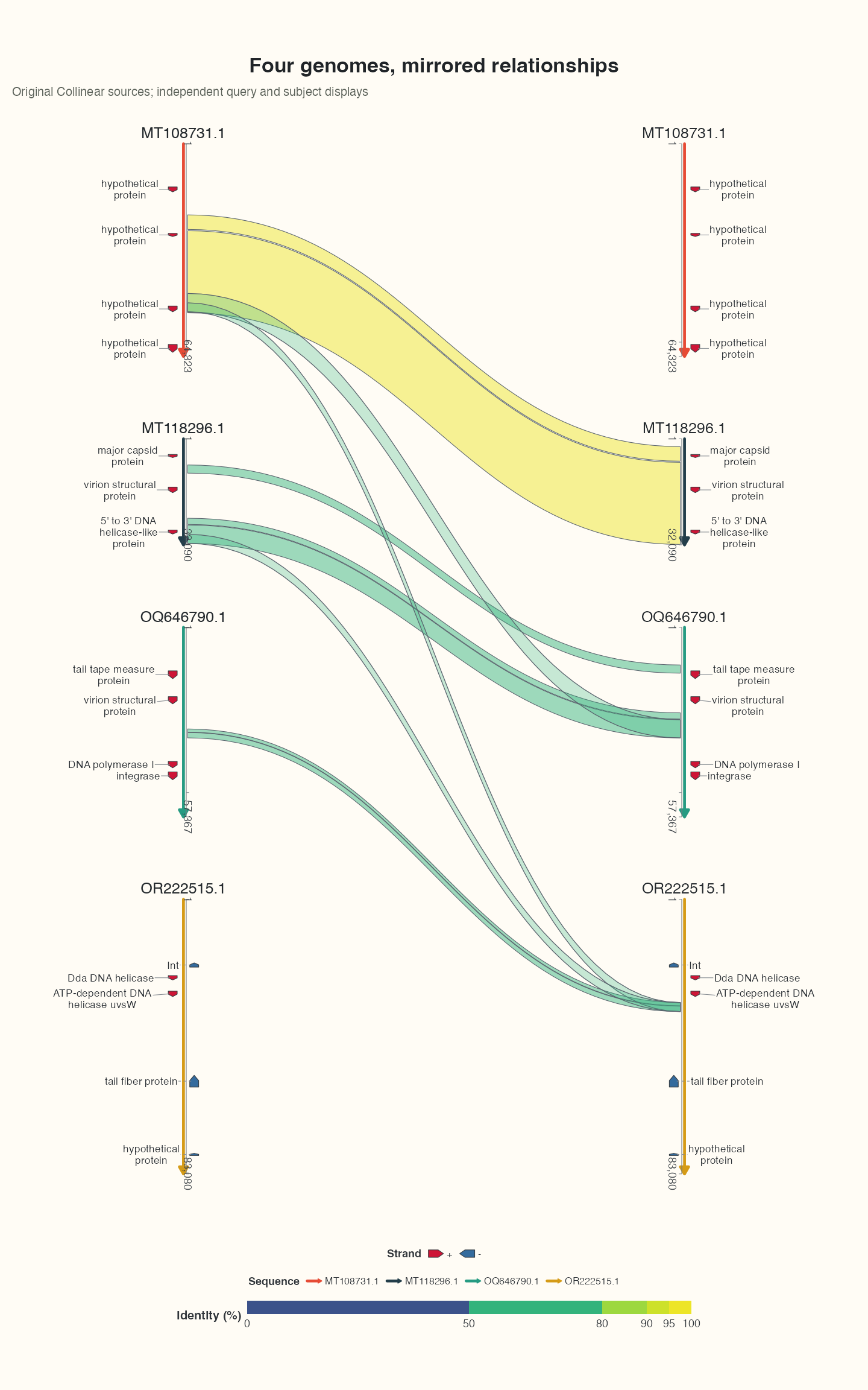
4 方向、实例与显示比例
生物学链、HSP 端点方向、显示 orientation 和 seq_order 各有独立含义。Sankey 的左右副本不增加观测,区间宽度不是流量守恒。图层仅在共同支持范围内可复用。
5 显示长度与连接样式
length_mode="equal" 改变角度分配或直线跨度,保留原始长度、区间与局部轴。 sequence_display 导出源长度和投影系数。多序列等长显示不能使用共享绝对比例尺。 默认轴显示 1 与真实末位,中间刻度按可用物理空间选择;闭圆接缝合并两端。 显式 breaks 和 labels 优先。
准备数据与配置(展开)
R · 示例代码
library(dplyr)
foundation_source <- ribbon_data_example |>
  mutate(source_hsp_id = paste0("bundled:", row_number()))
foundation_pair <- foundation_source |>
  slice_head(n = 1) |>
  select(qaccver, saccver)
foundation_ids <- c(foundation_pair$qaccver, foundation_pair$saccver)
foundation_seqs <- seq_data_example |>
  filter(accver %in% foundation_ids) |>
  select(accver, length)
foundation_hsp <- foundation_source |>
  filter(qaccver %in% foundation_ids, saccver %in% foundation_ids,
    qaccver != saccver)
foundation_features <- gene_data_example |>
  filter(accver %in% foundation_ids) |>
  transmute(accver, start, end, strand = source_strand, anno)
R · 示例代码
p_foundationequal <- ggchord(foundation_seqs, foundation_hsp) +
  geom_seq(length_mode = "equal") +
  geom_link_ribbon(aes(ribbon_fill = pident), tip = "none") +
  coord_collinear()
view_ggchord(p_foundationequal, width = 9, height = 5, units = "in")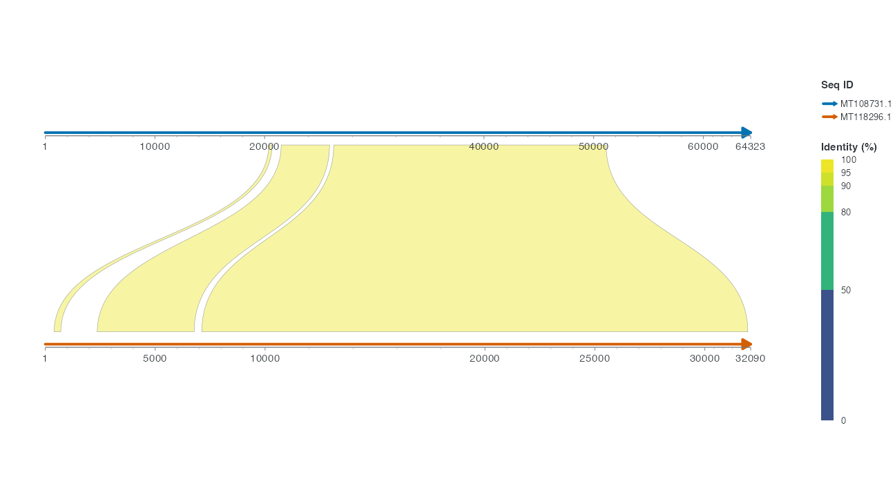
默认 Ribbon 使用 Identity 填充并保留完整区间端面;显式 geom_link_ribbon(gradient = TRUE) 才沿曲线插值端点序列色。tip="subject" 才在 subject 端装饰性收尖, 箭肩保留平移后的目标端点跨度,尖点不代表唯一匹配碱基或生物学转移方向; 源端点仍在布局导出中。tip="none" 保留完整端面。固定 fill、ribbon_fill 映射或显式 Ribbon 填充标度会覆盖显式启用的端点插值。显式 pident 使用固定 0–100 域,边界为 0/50/80/90/95/100,五段数值比例为 50/30/10/5/5%。用户标度与 guide 优先。
5.1 可选 subject 收尖
R · 示例代码
p_foundationarrow <- ggchord(foundation_seqs, foundation_hsp) +
  geom_seq() +
  geom_link_ribbon(tip = "subject") +
  coord_collinear()
view_ggchord(p_foundationarrow, width = 9, height = 5, units = "in")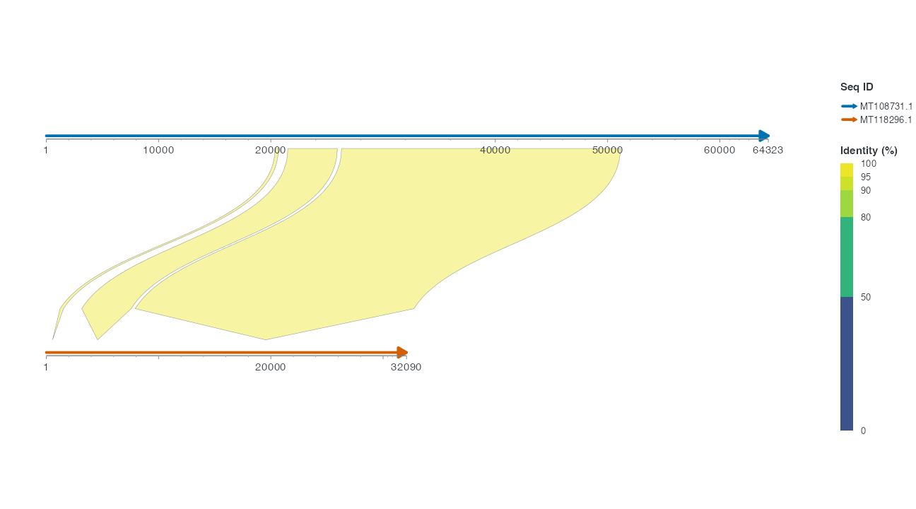
自动离散图例测量文字后选择行列,渲染循环联合测量图例与 panel;显式 guide/theme 设置优先。圆图外侧标签在所有数量下共享测量队列,label_visibility 报告源行、可见性 及可用的放置字段。未测得碰撞数不等于零。过小画布仍可能拥挤,请按目标导出尺寸 检查输出诊断。
自动 Identity 标尺按边界文字的实际尺寸预留长度,不再把通用色块尺寸当成整条标尺长度。手动指定长度时,使用 legend.ribbon.key.height、legend.ribbon.key.width 或显式 guide。圆图 parallel 坐标轴文字逐字符沿圆弧排布;水平和数值角度仍保留直线文字。
6 操作示例
选一条 HSP,指出两端来源;恢复默认邻接后说明为何可能省略。按目标尺寸保存选定视图,保留输入表。