Site guide · find your task
Quantitative tracks
On this page
Compute GC fractions from real DNA, then add bars, a moving mean and an annotation band. Each track has an explicit unit, window and baseline.
Prepare this page
In a fresh R session, run the code below, then follow this page in order. Colours and layout are optional display choices; inputs select only the fields needed.
Preparation code — run once on this page
Code
library(ggchord)
feature_palette <- c(
  CDS = "#993366", promoter = "#31849B", rep_origin = "#F1E51D",
  primer_bind = "#A020F0", misc_feature = "#A6ACB3", protein_bind = "#31849B"
)

library(ggchord)
doc_background <- "#FFFCF5"
identity_palette <- c("#303B71", "#36537D", "#269B82", "#A5D52C", "#ECEB31")
identity_values <- c(0, 0.5, 0.8, 0.9, 1)
identity_breaks <- c(0, 50, 80, 90, 100)
doc_legend_theme <- theme(
  legend.title = element_text(size = 13, face = "bold"),
  legend.text = element_text(size = 11),
  legend.key.width = unit(9, "mm"), legend.key.height = unit(5, "mm"),
  legend.spacing.x = unit(9, "mm"), legend.spacing.y = unit(7, "mm"),
  legend.margin = margin(l = 4, r = 4, unit = "mm")
)
sequence_guide <- guide_ggchord_legend(nrow = 1, theme = doc_legend_theme)
strand_guide <- guide_ggchord_legend(
  nrow = 1, override.aes = list(strand = c("+", "-")), theme = doc_legend_theme
)
identity_guide <- guide_ggchord_colourbar(
  position = "left", direction = "vertical",
  theme = theme(
    legend.key.height = unit(75, "mm"), legend.key.width = unit(5, "mm"),
    legend.title = element_text(size = 13, face = "bold"),
    legend.text = element_text(size = 11), legend.margin = margin(r = 7, unit = "mm")
  )
)
doc_theme <- theme_ggchord_publication(
  axis.text = element_text(size = 11),
  axis.text.check.overlap = TRUE
) +
  theme(
    legend.position = "bottom",
    legend.title = element_text(size = 13, face = "bold"),
    legend.text = element_text(size = 11),
    legend.key.width = unit(9, "mm"), legend.key.height = unit(5, "mm"),
    legend.spacing.x = unit(9, "mm"), legend.spacing.y = unit(7, "mm"),
    legend.box.spacing = unit(6, "mm"),
    plot.background = element_rect(fill = doc_background, colour = NA),
    panel.background = element_blank(),
    plot.title = element_text(face = "bold", size = 18),
    plot.subtitle = element_text(size = 10, colour = "#5C625A"),
    plot.margin = margin(14, 18, 14, 18)
  )
doc_axis <- function(coordinates = "relative") {
  scale_seq_position_continuous(
    coordinates = coordinates, n.breaks = 3, minor_breaks = NULL,
    labels = function(x) format(x, scientific = FALSE, big.mark = ",", trim = TRUE)
  )
}

library(dplyr)
data(plasmid_example_pUC19)
plasmid_seq <- plasmid_example_pUC19 |>
  select(accver, length)
feature_source <- find_common_features(plasmid_example_pUC19)
features <- feature_source |>
  select(accver, start, end, strand, type, anno)
Compute a track from actual DNA
After this page’s preparation code, compute GC fraction in 100 bp windows of bundled pUC19. The final shorter window uses its actual base count.
Code
library(dplyr)
data(plasmid_example_pUC19)
track_seq <- plasmid_example_pUC19 |>
  select(accver, length)
starts <- seq.int(1L, track_seq$length, by = 100L)
gc_fraction <- function(sequence) {
  bases <- strsplit(sequence, "")[[1]]
  mean(bases %in% c("G", "C"))
}
bins <- tibble(
  accver = track_seq$accver,
  start = starts,
  end = pmin(starts + 99L, track_seq$length)
) |>
  rowwise() |>
  mutate(gc = gc_fraction(substr(plasmid_example_pUC19$sequence, start, end))) |>
  ungroup()
head(bins)
Each row of bins is an actual sequence window. Check its endpoints and gc, then map values to track height and colour.
Draw GC fractions
Code
p_tracks <- ggchord(seq_data = track_seq) +
  geom_seq() +
  geom_seq_center_label() +
  geom_track_bar(aes(track_value = gc, track_fill = gc),
    data = bins,
    position = position_track("gc", width = unit(10, "mm"))
  ) +
  scale_track_value_continuous("gc", limits = c(0, 1), unit = "GC fraction") +
  scale_track_fill_gradientn("gc", colours = c("#E4F3EA", "#65B79B", "#27775C")) +
  coord_circular() +
  doc_theme
p_tracks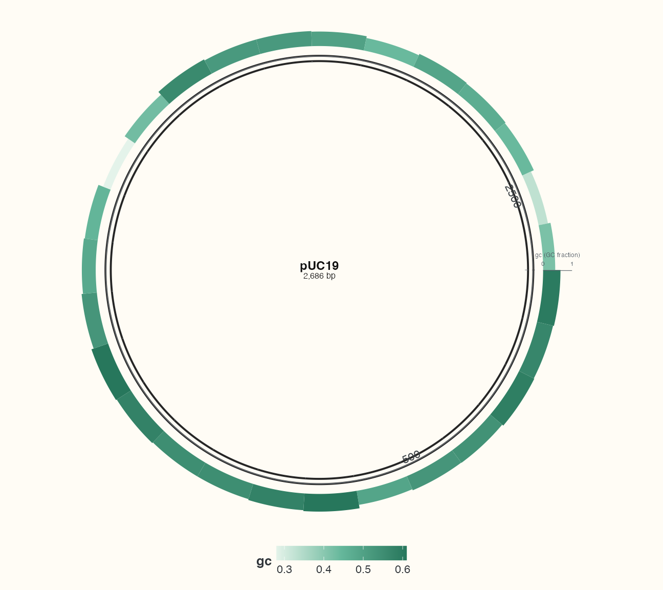
The domain is 0–1, in fractions. Replace it with the actual unit/range of other measurements. position_track() controls placement/physical width; scale_track_value_continuous() controls numerical mapping.
Share an ID deliberately
Same-ID layers share a numerical domain, including bar baselines, and must agree on width/placement. Colour scales are scoped independently by track ID. Tiles show interval categories, lines connect observations, bars encode interval values relative to a baseline. Sharing a domain does not require sharing a spatial band.
Inspect retention and limits
The export’s track_registry and track_diagnostics record domains, physical sizes, native offsets and clipping. Omitted/clipped rows do not mean zero values. Focus tracks with focus_ggchord_track() using the same windows.
Combine bars, a moving mean and annotation bands
Run the circular example to obtain real features first.
Code
line_bins <- bins |>
  transmute(
    accver,
    pos = floor((start + end) / 2),
    gc_mean = as.numeric(stats::filter(gc, rep(1 / 3, 3), sides = 2))
  ) |>
  filter(is.finite(gc_mean))
categories <- features |>
  select(accver, start, end, type)
p_multitrack <- ggchord(seq_data = track_seq) +
  geom_seq() +
  geom_seq_center_label() +
  geom_track_bar(aes(track_value = gc, track_fill = gc),
    data = bins,
    position = position_track("gc", width = unit(10, "mm"))
  ) +
  geom_track_line(aes(track_value = gc_mean),
    data = line_bins,
    position = position_track("gc", width = unit(10, "mm")), colour = "#233E4A"
  ) +
  scale_track_value_continuous("gc", limits = c(0, 1), unit = "GC fraction") +
  scale_track_fill_gradientn("gc", colours = c("#E4F3EA", "#65B79B", "#27775C")) +
  geom_track_tile(aes(track_fill = type),
    data = categories,
    position = position_track("features", order = 2, width = unit(2, "mm"))
  ) +
  scale_track_fill_manual("features", values = feature_palette) +
  coord_circular() +
  doc_theme +
  theme(legend.box = "vertical", legend.box.just = "left")
focused_bins <- focus_ggchord_track(bins, track_seq,
  loci = tibble(accver = track_seq$accver, start = 500, end = 1500), type = "interval"
)
p_multitrack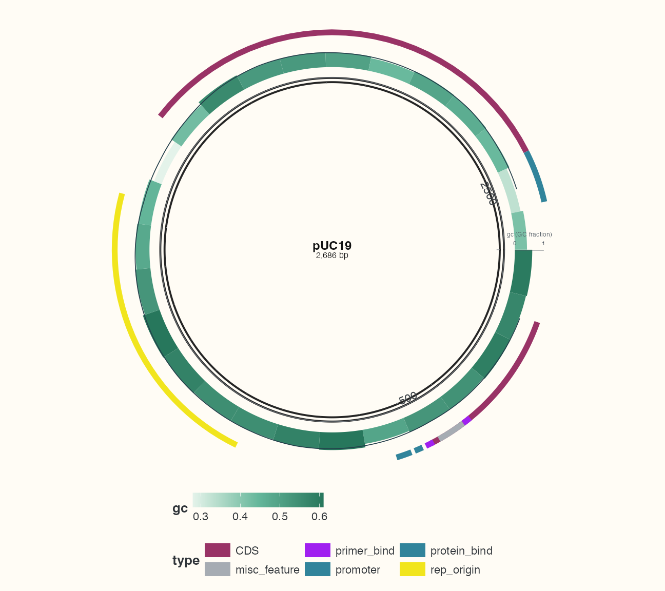
Bars and line use the same actual GC measurements; the line is a three-window moving mean. Incomplete end windows are omitted, not filled with invented values. Line positions use integer bin midpoints. Annotation bands have an independent ID and palette. Bands are explicitly ordered outside; overly wide inner bands at small radii can fold and are rejected.
Check your result
GC in bins lies between 0 and 1; each row is an actual window and the last may be shorter than 100 bp. Continuous colour expresses values; the category band expresses feature types, not GC magnitude.
Save this result
Save the plot just created to the working directory; use matching dimensions for preview.
Code
ggsave("pUC19-tracks.png", p_multitrack, width = 9, height = 8, units = "in", dpi = 144)