Chapters and reference
Module I · Multi-sequence relationships · Section 5 of 16
1.4 Intervals, points and cross-row links
On this page
- 1 Change where a ribbon passes
- 2 Compare clearance around a real CDS
- 3 Link two positions and highlight an interval
- 4 Branches, filtering and fixed-style boundaries
- 5 Cross-row links
- 6 Allow a cross-row link
- 7 Set the cross-row outline width
- 8 Shared branches and point links
- 9 Prepare an illustrative shared endpoint
- 10 Independent ribbons and a shared query trunk
- 11 Change the trunk fraction
- 12 Replace intervals with points
- 13 Real inputs and coordinate choices
- 14 Choose interval ribbons or point links
Data preparation and settings (expand)
R · Example code
p_chord_backbone <- ggchord(seq_data = seq_data_example) +
  geom_seq() +
  geom_seq_label() +
  coord_chord()
R · Example code
chord_links <- head(ribbon_data_example, 1)1 Change where a ribbon passes
R · Example code
p_chord_backbone <- ggchord(seq_data = seq_data_example) +
  geom_seq() +
  geom_seq_label() +
  coord_chord()

chord_links <- head(ribbon_data_example, 1)

p_chord_ribbon <- p_chord_backbone +
  geom_link_ribbon(data = chord_links)
view_ggchord(p_chord_ribbon, width = 7, height = 7, units = "in")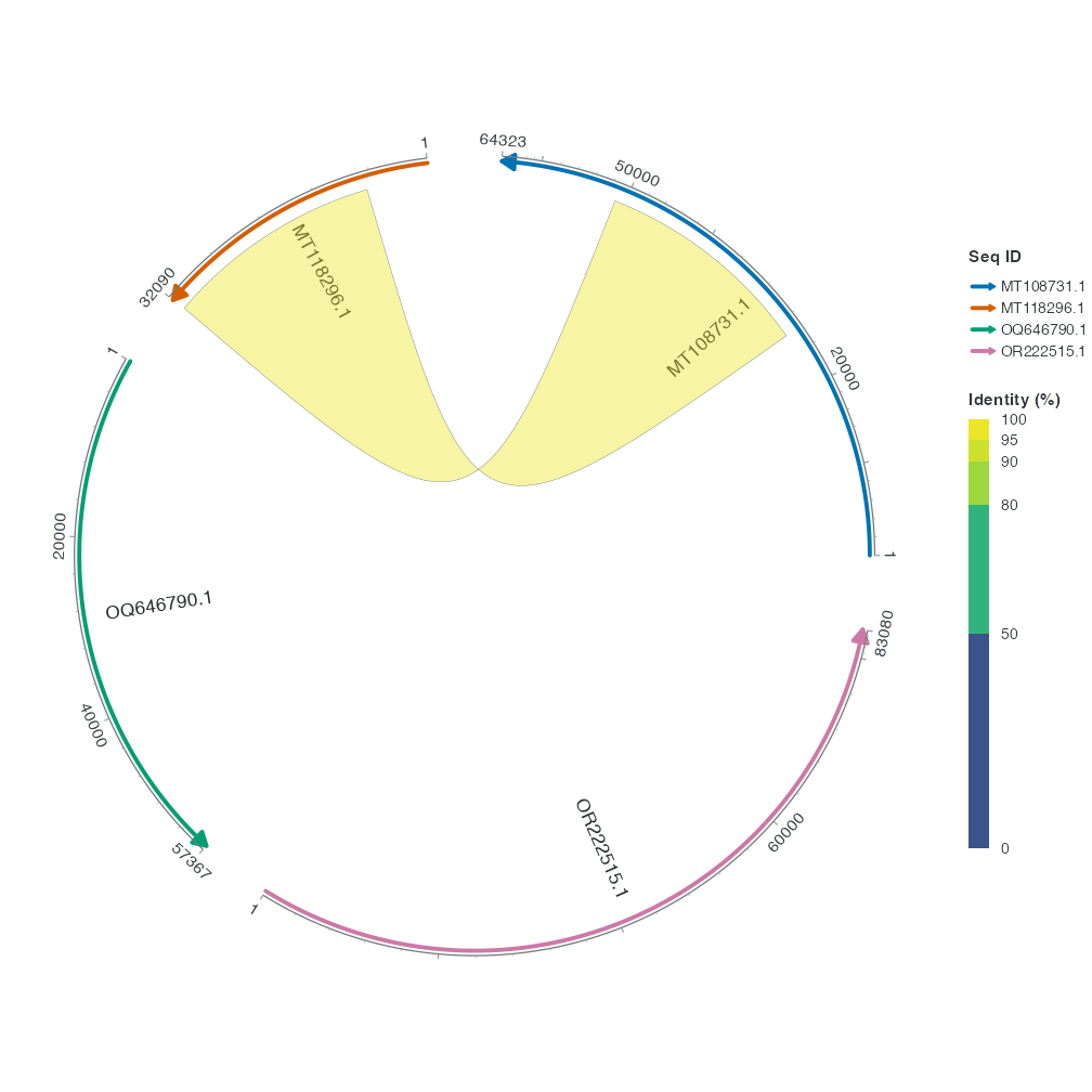
The default control is at the layout origin. Set link_ctrl_point to c(0, 0.8) to move the control upward in layout coordinates. Compare the path through the middle. Both ribbon ends still mark the same intervals.
R · Example code
p_chord_route <- p_chord_backbone +
  geom_link_ribbon(data = chord_links, link_ctrl_point = c(0, 0.8))
view_ggchord(p_chord_route, width = 7, height = 7, units = "in")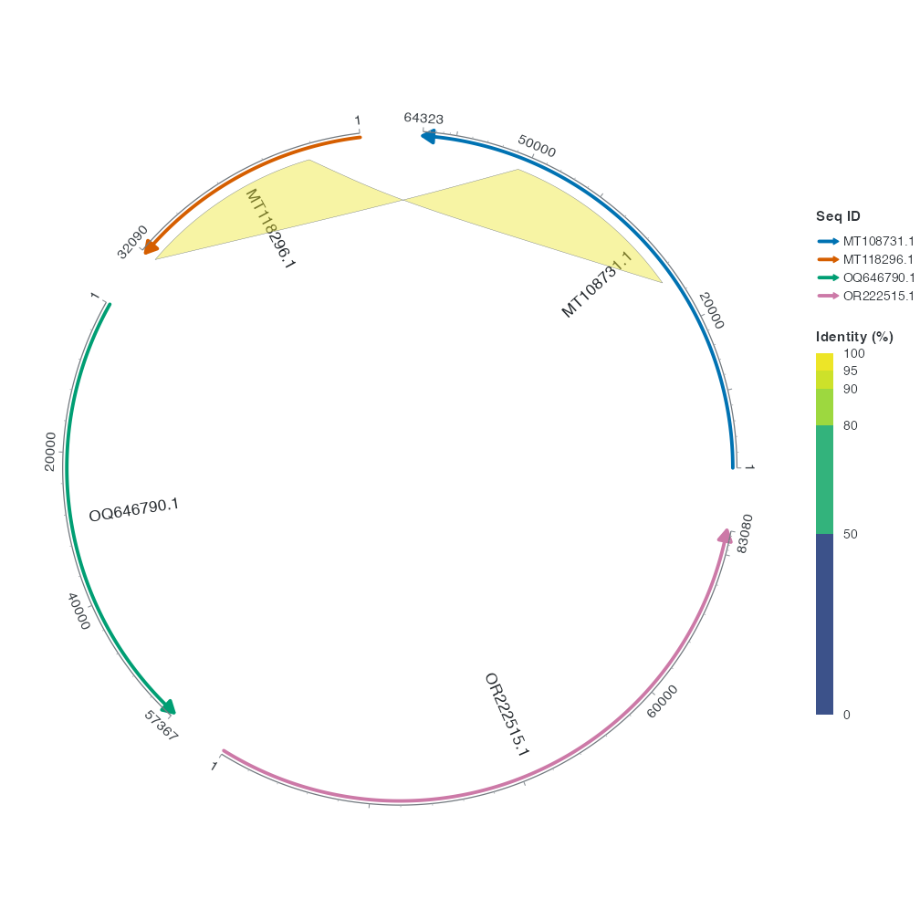
Control points use unrotated layout coordinates. With the default rotation of 0°, (0, 0.8) pulls the ribbon upwards. Rotating the whole layout also rotates the control point. A Bézier control pulls the curve without generally lying on it.
2 Compare clearance around a real CDS
Take the CDS at 48,053–49,111 bp on MT108731.1. It falls within the alignment’s query interval. Move the plus-strand arrow inward by 0.05 layout units so it sits on the ribbon side of the backbone.
R · Example code
chord_obstacle <- subset(gene_data_example, accver == "MT108731.1" & start == 48053)
chord_obstacle$strand <- chord_obstacle$source_strand
p_chord_obstacle <- p_chord_backbone +
  geom_gene(data = chord_obstacle, position = position_strand(c("+" = -0.05)))

p_chord_no_avoid <- p_chord_obstacle +
  geom_link_ribbon(data = chord_links, link_avoid = "none")
view_ggchord(p_chord_no_avoid, width = 7, height = 7, units = "in")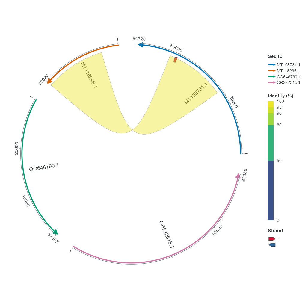
link_avoid = "none" uses fixed endpoint clearance. Look near 49 kb on the MT108731.1 backbone, where the ribbon overlaps part of the arrow.
R · Example code
p_chord_smooth <- p_chord_obstacle +
  geom_link_ribbon(data = chord_links, link_avoid = "smooth")
view_ggchord(p_chord_smooth, width = 7, height = 7, units = "in")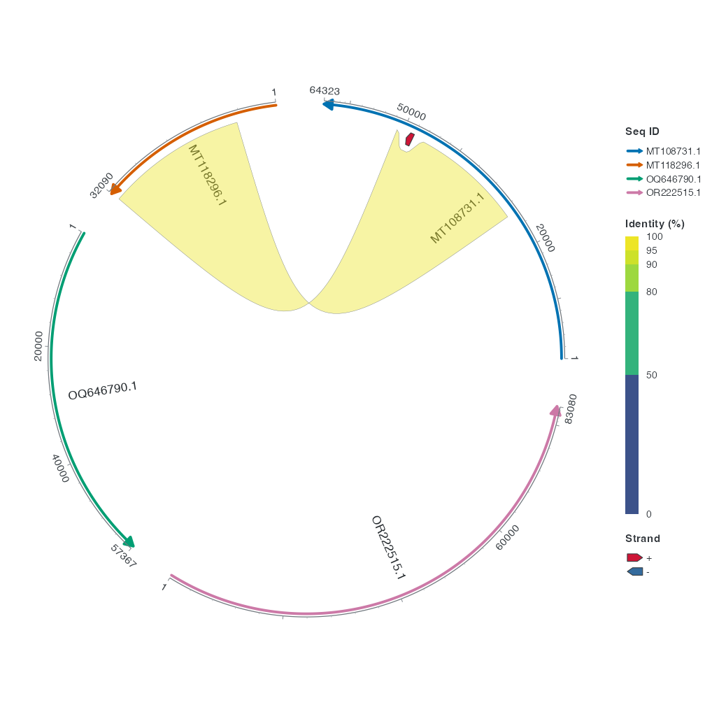
link_avoid = "smooth" increases clearance locally near the CDS. At the same spot on the MT108731.1 backbone, the ribbon edge recedes to leave space for the arrow. The default "uniform" applies one clearance across each endpoint interval. A numeric link_gap sets the spacing directly.
3 Link two positions and highlight an interval
R · Example code
chord_query_region <- data.frame(
  accver = chord_links$qaccver, start = chord_links$qstart, end = chord_links$qend
)
chord_midpoints <- transform(chord_links,
  qpos = floor((qstart + qend) / 2), spos = floor((sstart + send) / 2)
)
p_chord_markers <- p_chord_backbone +
  geom_seq_region(data = chord_query_region, region_side = "outside") +
  geom_link_line(data = chord_midpoints, link_type = "straight",
                 arrow = grid::arrow(length = grid::unit(2, "mm")))
view_ggchord(p_chord_markers, width = 7, height = 7, units = "in")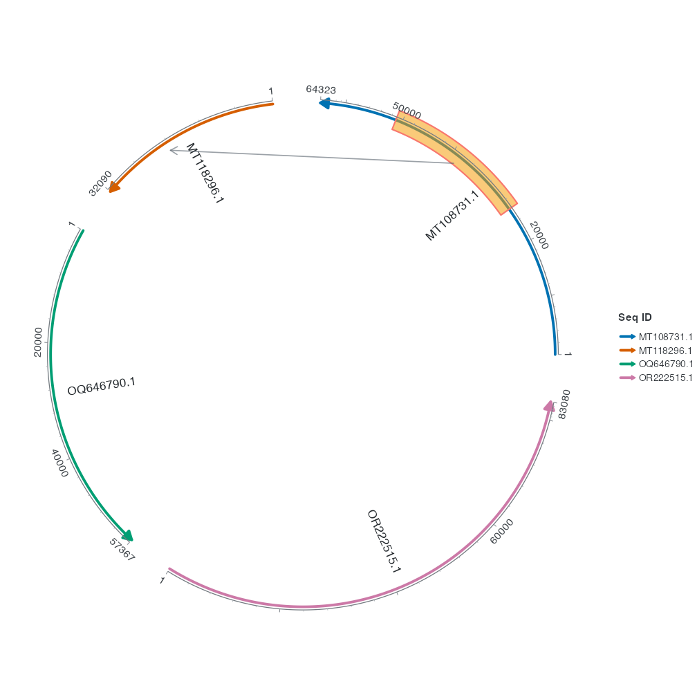
The outer band marks the full interval on the query sequence. region_side = "outside" places it outside the backbone. The straight line joins the two interval midpoints, and the arrow points to the subject. Use a ribbon to show the full span on both sides.
Next, place sequence and gene labels.
4 Branches, filtering and fixed-style boundaries
| Parameter | Current default | When to change and constraints |
|---|---|---|
link_branch |
"none" |
query/subject share trunks for equal endpoints; unequal endpoints do not establish homology |
link_branch_fraction |
0.15 |
Trunk length relative to the shortest member, in (0, 0.5]; only meaningful with branching |
pairs |
NULL |
Explicit sequence-pair selection; does not create alignments |
link_gap |
NULL |
Uses avoidance policy; an explicit number overrides automatic clearance |
link_avoid |
"uniform" |
none uses fixed clearance, smooth local avoidance; text and leaders are ignored |
link_ctrl_point |
NULL |
Origin in chord mode; endpoint-derived in collinear mode; not bp coordinates |
nonadjacent_linewidth |
0.4 |
Only nonadjacent collinear borders; 0 reuses ordinary linewidth |
Set fixed fill/alpha/colour/linewidth outside aes(). Map data differences to dedicated ribbon roles with matching scales. Explicit fixed values override matching mappings; omit fixed alpha when mapping opacity. Colour differences do not establish biological relationships. See geom_link_ribbon() for the full signature.
Continue with shared branches and point links to compare trunks, trunk fractions and curved/straight paths.
5 Cross-row links
Data preparation and settings (expand)
R · Example code
p_linear_base <- ggchord(seq_data = seq_data_example) +
  geom_seq() +
  geom_seq_label() +
  coord_collinear()
R · Example code
chord_links <- head(ribbon_data_example, 1)R · Example code
p_linear_link <- p_linear_base + geom_link_ribbon(data = chord_links)6 Allow a cross-row link
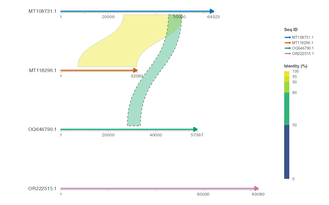
Only Collinear uses thin solid outlines for adjacent rows and heavier dashed outlines for cross-row ribbons. Chord, Radial and Sankey use ordinary solid outlines by default. linewidth controls the ordinary width; nonadjacent_linewidth separately controls cross-row width and defaults to 0.4.
The second ribbon layer receives one alignment between the first and third rows. Set adjacent_only = FALSE to show it. The default dashed outline marks the skipped row. The original ribbon between rows one and two stays in its own layer.
7 Set the cross-row outline width
R · Example code
p_cross_width <- p_linear_link +
  geom_link_ribbon(data = cross_link, adjacent_only = FALSE,
    nonadjacent_linewidth = 0.8)
view_ggchord(p_cross_width, width = 8, height = 5, units = "in")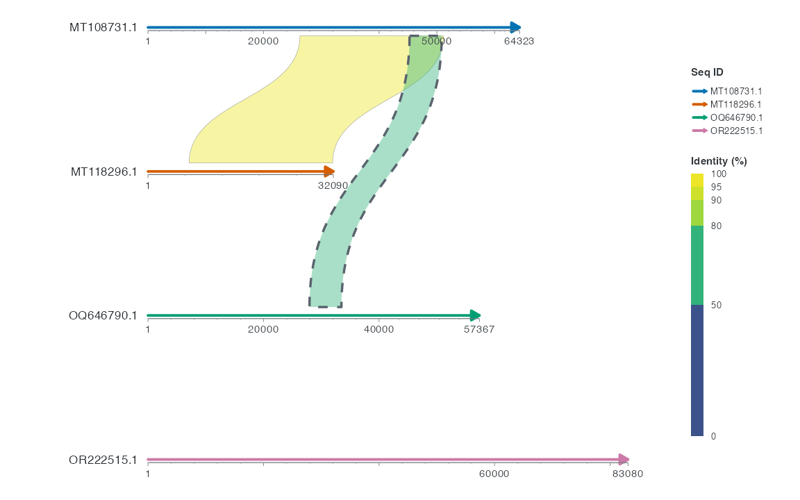
nonadjacent_linewidth = 0.8 thickens the second layer’s cross-row ribbon. The first layer’s adjacent ribbon and both line types are retained.
R · Example code
p_cross_same <- p_linear_link +
  geom_link_ribbon(data = cross_link, adjacent_only = FALSE,
    linewidth = 0.2, nonadjacent_linewidth = 0)
view_ggchord(p_cross_same, width = 8, height = 5, units = "in")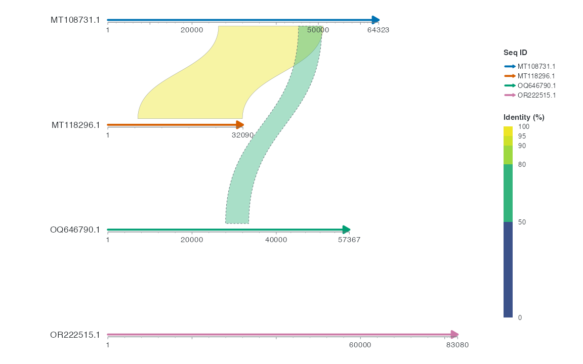
Zero uses the layer’s ordinary linewidth, here 0.2. The outline remains dashed. When using aes(linewidth = ...), the mapping and scale control the widths.
8 Shared branches and point links
9 Prepare an illustrative shared endpoint
R · Example code
library(ggchord)
branch_seqs <- data.frame(accver = c("query", "target_a", "target_b"), length = 1000)
branch_links <- data.frame(
  qaccver = c("query", "query"), saccver = c("target_a", "target_b"),
  qstart = 200, qend = 600, sstart = c(100, 300), send = c(500, 700)
)
branch_base <- ggchord(branch_seqs, ribbon_data = branch_links) +
  geom_seq() + geom_seq_label() + coord_chord(rotation = 0)
Three illustrative sequences each span 1000 bp. Two links share query interval 200–600 bp and connect to different target intervals. Coordinates are one-based inclusive. Every figure uses 9 × 7 inches; endpoints stay fixed across branch settings.
10 Independent ribbons and a shared query trunk
R · Example code
p_comparebranchnone <- branch_base + geom_link_ribbon(link_branch = "none")
view_ggchord(p_comparebranchnone, width = 9, height = 7, units = "in")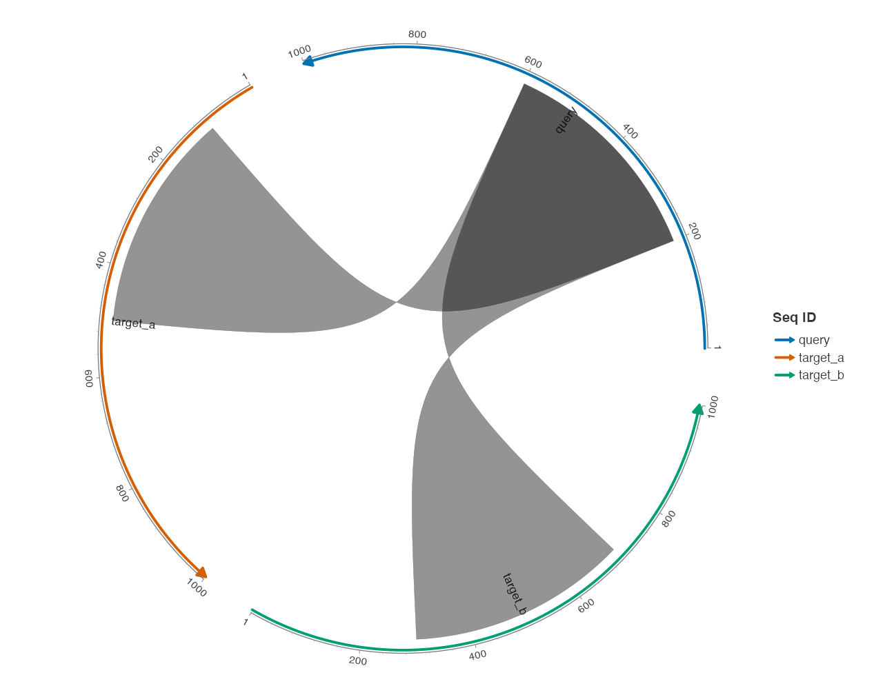
With default link_branch = "none", the ribbons travel independently and may overlap near the query end.
R · Example code
p_comparebranchquery <- branch_base + geom_link_ribbon(link_branch = "query")
view_ggchord(p_comparebranchquery, width = 9, height = 7, units = "in")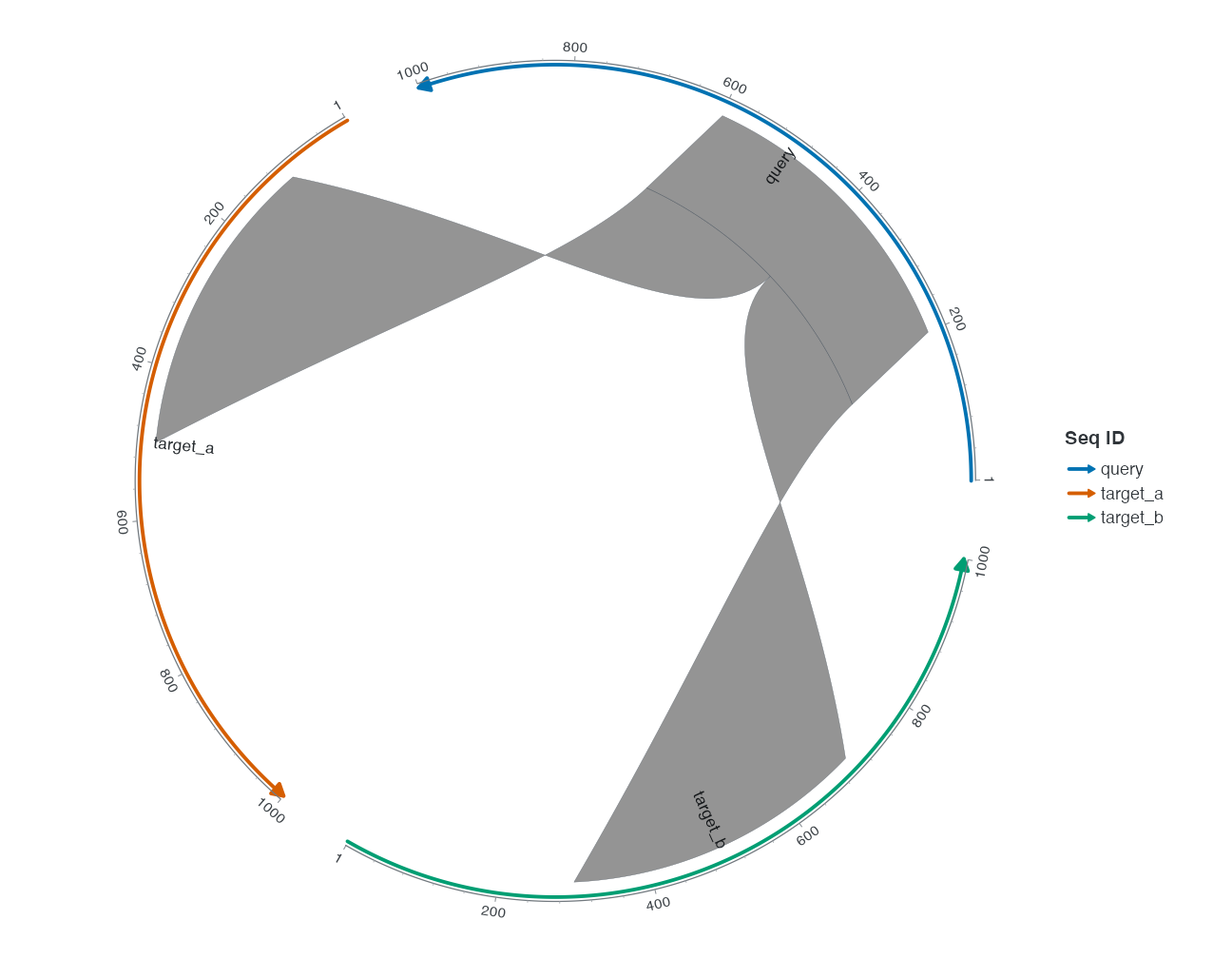
Only change to "query": equal query endpoints can share a trunk. Overlapping intervals are not necessarily equal endpoints. Real data without suitable groups may show no change when branching is enabled. "subject" groups equal subject endpoints instead.
11 Change the trunk fraction
R · Example code
p_comparebranchfraction <- branch_base +
  geom_link_ribbon(link_branch = "query", link_branch_fraction = 0.35)
view_ggchord(p_comparebranchfraction, width = 9, height = 7, units = "in")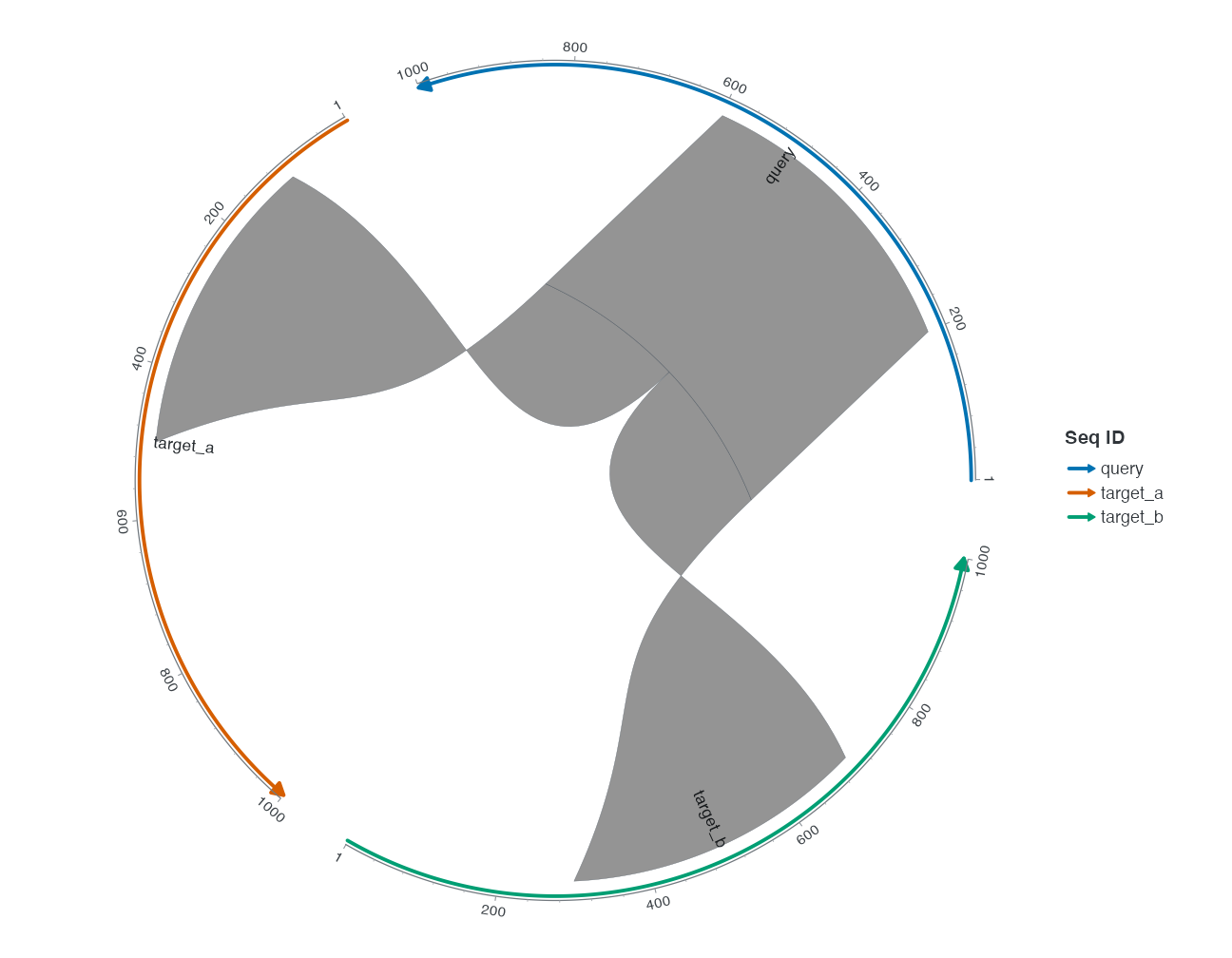
Relative to the query-branch figure, only link_branch_fraction changes from default 0.15 to 0.35. The shared trunk becomes longer relative to the shortest member. It is not identity, a probability or a newly measured alignment length.
| Parameter | Default | Effect and constraints |
|---|---|---|
link_branch |
"none" |
none/query/subject; selects the shared endpoint |
link_branch_fraction |
0.15 |
In (0, 0.5]; none does not create a shared trunk |
link_ctrl_point |
NULL |
Shapes far ends when branching; the trunk determines its junction |
pairs |
NULL |
qaccver/saccver table selecting existing pairs, not generating alignments |
12 Replace intervals with points
Point links require explicit qpos/spos; an interval table is not a point table. Here choose interval midpoints. This loses interval length encoded by ribbon width, so explain the selection rule first.
R · Example code
point_links <- data.frame(
  qaccver = branch_links$qaccver, saccver = branch_links$saccver,
  qpos = (branch_links$qstart + branch_links$qend) / 2,
  spos = (branch_links$sstart + branch_links$send) / 2
)
R · Example code
p_comparelinkcurve <- branch_base + geom_link_line(data = point_links, link_type = "curve")
view_ggchord(p_comparelinkcurve, width = 9, height = 7, units = "in")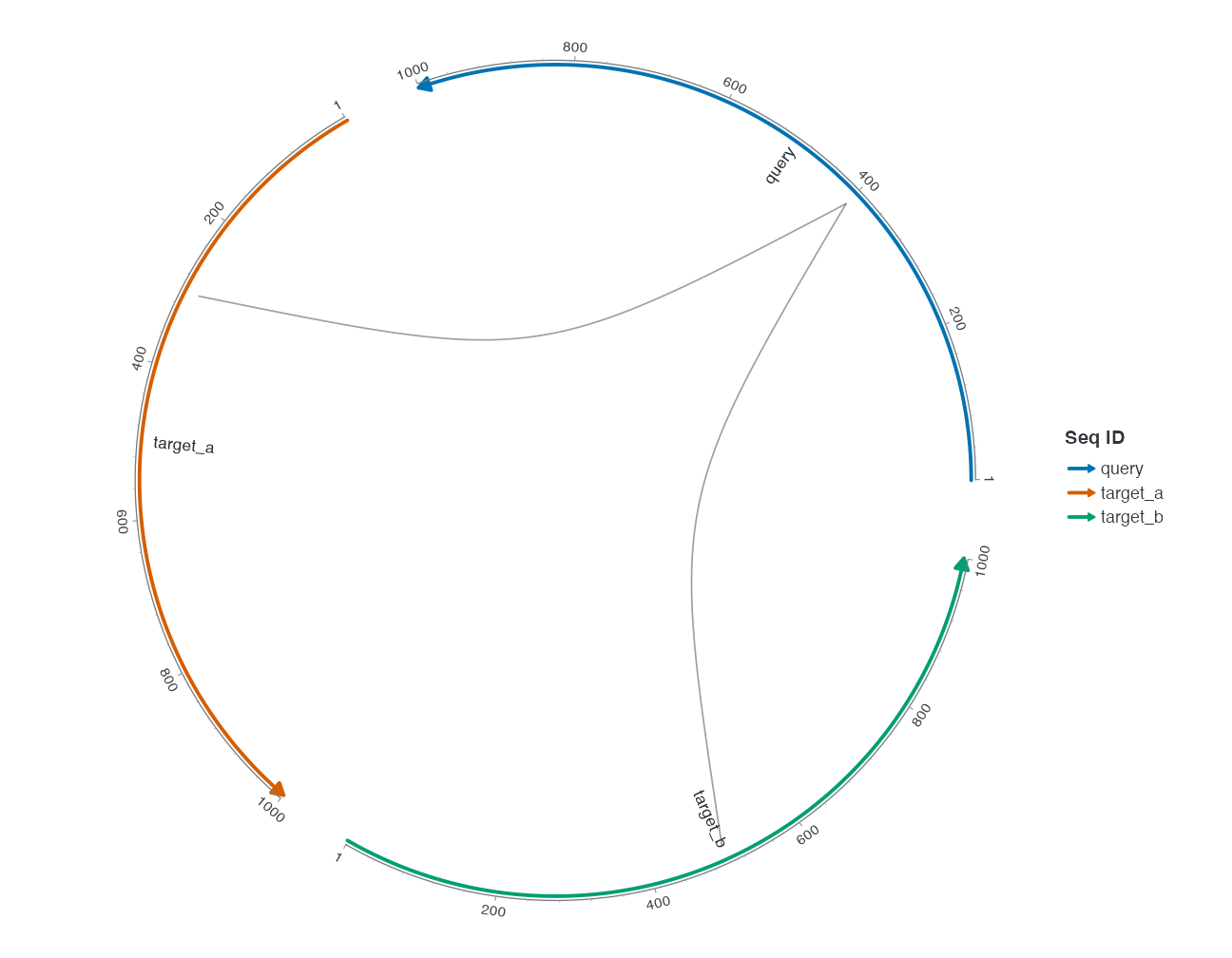
Default link_type = "curve" connects the selected positions with curves.
R · Example code
p_comparelinkstraight <- branch_base + geom_link_line(data = point_links, link_type = "straight")
view_ggchord(p_comparelinkstraight, width = 9, height = 7, units = "in")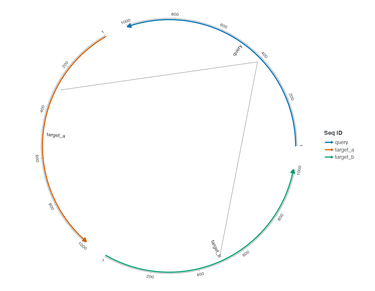
Only change to "straight", keeping input, anchors and dimensions fixed. Add arrow = grid::arrow() separately for direction. It represents the query-to-subject drawing convention, not independent evidence of gene strand or transcription.
13 Real inputs and coordinate choices
Preserve real query/subject endpoints. Do not edit unequal endpoints to manufacture shared trunks. See link preparation for filtering and bundling; geometric branching does not perform those statistics.
Chord and collinear modes accept these link layers; single circular mode rejects ribbon/link. Linear adjacency filtering still applies. Check adjacent_only or explicit pairs before showing cross-row ribbons; see cross-row links.
Example: change only the trunk fraction to 0.25. Return to the default fraction and compare curved versus straight point links. With your own data, first decide whether interval lengths or individual positions matter, then consult geom_link_ribbon() and geom_link_line().
Data preparation and settings (expand)
R · Example code
ribbon_sequences <- seq_data_example
observed_links <- ribbon_data_example
14 Choose interval ribbons or point links
R · Example code
points <- transform(head(observed_links, 3),
  qpos = floor((qstart + qend) / 2),
  spos = floor((sstart + send) / 2)
)
p_points <- ggchord(seq_data = ribbon_sequences) +
  geom_seq() +
  geom_link_line(data = points, arrow = grid::arrow(length = grid::unit(2, "mm"))) +
  coord_chord()
view_ggchord(p_points, width = 10, height = 8, units = "in")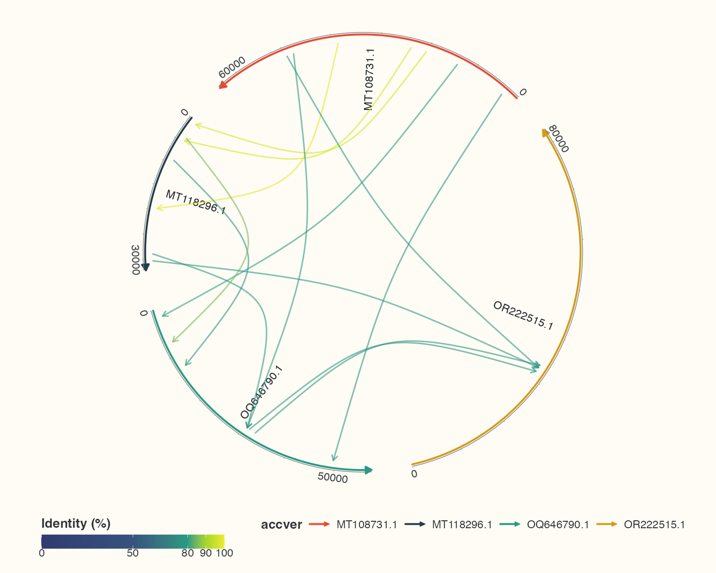
These arrows join the midpoints of the first three alignments and point toward the subject. Use ribbons to show complete intervals.