Chapters and reference
Data and workflows · Section 5 of 12
6.4 Aligned characters and source coordinates
On this page
Data preparation and settings (expand)
R · Example code
library(dplyr)
seqs <- seq_data_example |>
  select(accver, length)
links <- ribbon_data_example |>
  select(qaccver, saccver, qstart, qend, sstart, send)
# Recover biological strands from the source annotation field.
genes <- gene_data_example |>
  transmute(accver, start, end, strand = source_strand)
The examples use bundled data and require no input download or extraction; optional dependencies are listed in each section. Original records remain traceable through the real input bundle.
1 Retain actual FASTA characters
Bundled sequence_detail_example$plasmid_source already retains real characters, physical header line numbers and source-file provenance; use keep_sequence = TRUE when importing your own FASTA. Import removes whitespace while retaining case; declare bp or aa explicitly rather than guessing the alphabet. Focusing clips both strings and intervals: local position 1 below corresponds to source position 1001. Descending regions select the same interval without reverse-complementing it. Lengths alone cannot recover characters, and HSP endpoints cannot recover mismatch or gap columns. Gapped FASTA lengths include gaps; genomic use needs a separate alignment-column-to-source-position mapping.
R · Example code
character_source <- sequence_detail_example$plasmid_source
character_locus <- focus_ggchord_data(
  character_source,
  loci = data.frame(accver = character_source$accver, start = 1001, end = 1060)
)
character_locus$seq_data |>
  select(accver, length, sequence, .source_origin)
1.1 Import your own existing alignment
This subsection specifically demonstrates read_aligned_fasta(). Replace the path with an existing equal-length FASTA; the source example is available in the input bundle. Reading is skipped when the file is absent, and subsequent plots continue to use the bundled tables directly.
R · Example code
alignment_file <- "examples/alignment/opuntia-aligned.fasta"
if (file.exists(alignment_file)) {
  imported_alignment <- read_aligned_fasta(
    alignment_file, "DNA", source_file = TRUE
  )
}
2 Existing alignments: keep columns and source positions separate
The examples directly use prepared DNA/protein alignment tables in sequence_detail_example. Original Biopython records, upstream licenses, hashes and reproducible FASTA conversion rules remain in the source directory examples/alignment/. No alignment tools are run and complete record IDs and original characters are unchanged; rows and columns are selected explicitly.
read_aligned_fasta() reads one existing alignment. Declare DNA, RNA or AA; equal lengths alone do not establish homology. alignment_column includes - and . gaps, whose source_position is NA. Default positions count the ungapped input fragment from one; they are not complete-genome coordinates. Lowercase letters consume positions, so this reader must not be used as an A3M insertion parser.
R · Example code
aligned_dna <- sequence_detail_example$dna_alignment
selected_rows <- unique(aligned_dna$accver)[c(1, 3, 7)]
local_dna <- aligned_dna |>
  filter(accver %in% selected_rows, between(alignment_column, 321, 380))

map_alignment_position(local_dna, selected_rows[1], c(342, 343, 344))
map_alignment_position(local_dna, selected_rows[1], 343, inverse = TRUE)

p_characters <- ggplot2::ggplot(
  local_dna, aes(alignment_column, accver, label = symbol)
) +
  geom_residue(overflow = "error") +
  scale_fill_residue("DNA") +
  ggplot2::labs(x = "Alignment column", y = NULL) +
  ggplot2::theme_minimal()
view_ggchord(p_characters)
The first selected row has a gap at alignment column 343. Column lookup therefore returns matched = TRUE, is_gap = TRUE and a missing source position. Inverse lookup of source position 343 finds its actual alignment column, without interpolation. Positions removed by filtering return matched = FALSE; filtering never renumbers retained columns. map_alignment_position() selects an alignment-row ID even when a separately declared source ID differs.
geom_residue() is a standard Cartesian ggplot layer. Styles and user scales follow ggplot2. It measures glyphs against actual cell width and height at draw time: overflow = "error" requires readable letters; "tile" retains colour cells where text cannot fit, without shrinking fonts. Focus fewer columns or increase physical width to show letters. For example, save p_characters with ordinary ggsave(width = 12, height = 3.4, units = "in"); simply raising DPI adds no physical room. Discrete rows, identity/reverse position scales and Cartesian coordinates are supported; this layer does not directly project characters onto backbone Coords. A Cartesian character plot with explicit source mapping can be registered using register_ggchord_alignment() for Fusion character details.
Default residue plots join neighbouring cells continuously and use a 1:1 cell ratio unless coordinates were explicitly supplied. Dark bold sans-serif glyphs fit the cells at a uniform size, with a default readability floor of 3 mm. Without an explicit fill, label is mapped automatically and the data alphabet selects DNA/RNA/AA chemistry colours. Use scale_fill_residue() to select an alphabet or ggplot2::scale_fill_manual() to replace the colours. Explicit sizes, mappings, fixed colours and user coordinates take priority. Character legends are hidden by default; enable them with show.legend = TRUE.
2.1 Automatic line wrapping
Pass line_width = 50 to geom_residue() to display 100 bases as lines 1–50 and 51–100. This example reads the first 100 observed bases of MT108731.1. Row labels retain the original column ranges and the x axis shows the column within a line. Multiple sequences share the same breaks, and gaps still occupy columns. Original data, alignment columns and source positions are not renumbered.
R · Example code
genome <- genome_comparison_example$sequences |>
  filter(accver == "MT108731.1")
fragment <- setNames(substr(genome$sequence, 1, 100), genome$accver)
cells <- as_ggchord_alignment(fragment, "DNA",
  source_data = data.frame(accver = genome$accver, start = 1, strand = "+",
    sequence = genome$sequence))
wrapped <- ggplot2::ggplot(cells, aes(alignment_column, accver, label = symbol)) +
  geom_residue(line_width = 50, overflow = "error") +
  ggplot2::theme_minimal(base_size = 12) +
  theme(panel.grid = element_blank(), axis.text = element_text(colour = "#202020"))
view_ggchord(wrapped, width = 10, height = 2.5, units = "in")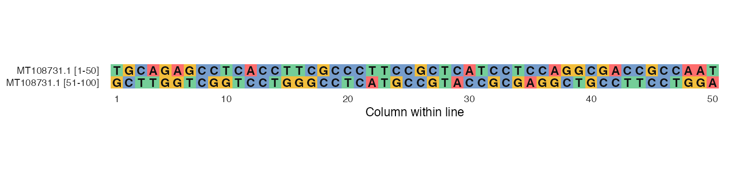
Wrapped character plots can also be registered for Fusion. Each focus interval must fit within one displayed line; split cross-line selections into explicit source intervals. The default line_width is NULL, which keeps a single line.
2.2 Protein excerpt
The same data contract accepts observed protein characters. The excerpt retains upstream gaps and residue differences; default fill groups amino acids by side-chain chemistry, rather than inferred functional domains.
R · Example code
aligned_protein <- sequence_detail_example$protein_alignment
protein_rows <- unique(aligned_protein$accver)[2:4]
local_protein <- aligned_protein |>
  filter(accver %in% protein_rows, between(alignment_column, 221, 260))

ggplot2::ggplot(local_protein, aes(alignment_column, accver, label = symbol)) +
  geom_residue(overflow = "tile") +
  ggplot2::labs(x = "Alignment column", y = NULL) +
  ggplot2::theme_minimal()
2.3 Explicit source coordinates
Provide one source_data row per aligned record with accver, start and strand. start is the first nongap source coordinate. Negative-strand positions decrease; strings must already be in alignment orientation. An optional source_accver identifies the original molecule. If you provide a full forward sequence, every nongap character is checked, using nucleotide complementation on the negative strand and order reversal only for AA. Missing source strings remain unverified; no origins or strands are guessed.
The following example checks consistency against ungapped fragments derived from the same alignment. It is deliberately not independent genomic validation. For a real genomic projection, supply independently known source sequences and interval metadata instead.
R · Example code
original_strings <- sequence_detail_example$aligned_strings
fragment_sources <- original_strings |>
  transmute(
    accver, source_accver = accver, start = 1, strand = "+",
    sequence = gsub("[-.]", "", sequence)
  )
checked_cells <- as_ggchord_alignment(
  original_strings, "DNA", source_data = fragment_sources
)
No mismatch/gap detail can be recovered from six HSP endpoints alone. This workflow accepts existing columns, not CIGAR/A3M/Clustal/Stockholm parsing, phase inference, consensus/Logo analysis or alignment computation. Explicit CDS translation is described below; exact macro/detail registration is available in the Fusion section.
3 Source-backed CDS translation
build_ggchord_cds() defines observed coding coordinates; translate_ggchord_cds() additionally needs actual complete forward DNA/RNA strings and optional Biostrings. This real EMALE negative-strand CDS has source phase 0 and an ATG start. Table 11 is an explicit choice checked against the unchanged upstream protein FASTA. Input provenance is in examples/format-inputs/README.md.
R · Example code
library(dplyr)
genome <- sequence_detail_example$coding_genome
coding <- sequence_detail_example$coding_features |>
  filter(feature_id == "BVI_023A_0009")
cds <- build_ggchord_cds(coding, genetic_code = 11)
observed <- translate_ggchord_cds(cds, genome, initiation = "start")
expected <- sequence_detail_example$coding_proteins |>
  filter(accver == "BVI_023A_0009")
stopifnot(sub("[*]$", "", observed$models$protein_sequence) == expected$sequence)
observed$residues |>
  select(alignment_column, symbol, codon, source_positions) |>
  head()
models reports coding/protein strings, genetic code, initiation/ambiguity policies, partial ends and terminal remainder. nucleotides retains each genomic base; residues$source_positions contains the three genomic positions of each codon in biological order, even across exon boundaries. Residue positions use the CDS feature ID’s observed-protein namespace; they are not an inferred external protein accession. Terminal and internal stops remain *. The example removes only the final stop for comparison with the upstream FASTA convention.
The default initiation = "literal" does not recode alternative starts; "start" requires a complete 5-prime end. ambiguous = "error" rejects fuzzy codons; explicit "solve" delegates to Biostrings, using X if unresolved. Unknown codes, missing/short sources and declared translation exceptions fail. partial = "trim" belongs to the CDS map: only the initial phase and incomplete terminal codon are excluded; later segment phases validate continuity without deleting junction bases. No missing sequence is reconstructed. RNA must be declared explicitly. Ordered segments support the existing spliced/origin-join contract.
A complete runnable nucleotide/codon/macro example is examples/m2-detail.R; its negative-strand labels are centred on their three coding bases. Real spliced plus/minus controls, source hashes and original expected translations are retained in examples/cds/. Register the character plot to connect its exact source boundaries.