Chapters and reference
Data and workflows · Section 8 of 12
6.7 BLASTp protein comparisons
On this page
Compare four complete proteins with two bundled tables, without downloading inputs or running BLASTp. Both backbones and alignment endpoints use amino-acid coordinates (aa).
1 Plot BLASTp protein alignments directly
protein_seq_data_example contains three EMALE proteins and one Mavirus protein. Inspect identifiers, full lengths and units:
R · Example code
protein_seq_data_example[c("accver", "length", "sequence_unit")]| accver | length | sequence_unit |
|---|---|---|
| BVI_029_0020 | 302 | aa |
| BVI_058_0011 | 302 | aa |
| E4-10_023_0015 | 306 | aa |
| ADZ16414.1 | 310 | aa |
The lengths are 302, 302, 306 and 310 aa, obtained from complete proteins rather than alignment endpoints. The sequence column retains complete residues; only the three plotting columns are shown here.
protein_ribbon_data_example contains six observed BLASTp comparisons between all four proteins. Inspect both interval endpoints and identity:
R · Example code
protein_ribbon_data_example[c("qaccver", "saccver", "qstart", "qend", "sstart", "send", "pident")]| qaccver | saccver | qstart | qend | sstart | send | pident |
|---|---|---|---|---|---|---|
| BVI_029_0020 | BVI_058_0011 | 1 | 302 | 1 | 302 | 99.007 |
| BVI_029_0020 | E4-10_023_0015 | 1 | 298 | 1 | 302 | 58.278 |
| BVI_029_0020 | ADZ16414.1 | 16 | 295 | 19 | 299 | 36.332 |
| BVI_058_0011 | E4-10_023_0015 | 1 | 298 | 1 | 302 | 58.609 |
| BVI_058_0011 | ADZ16414.1 | 16 | 295 | 19 | 299 | 36.897 |
| E4-10_023_0015 | ADZ16414.1 | 47 | 305 | 52 | 304 | 35.741 |
R · Example code
p_native_protein <- ggchord(protein_seq_data_example, protein_ribbon_data_example) +
  geom_seq() +
  geom_seq_label() +
  geom_link_ribbon() +
  geom_seq_scale(length = 50) +
  coord_collinear()
view_ggchord(p_native_protein, width = 8, height = 5, units = "in")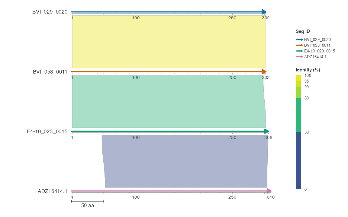
The collinear layout connects adjacent rows by default, displaying three ribbons. Colours show identity and the scale bar spans 50 aa. The first two proteins are highly similar; the remaining adjacent comparisons are weaker. Intervals are inclusive and retain both endpoint spans of gapped alignments.
Switching to a chord layout displays all six pairs by default:
R · Example code
p_native_chord <- ggchord(protein_seq_data_example, protein_ribbon_data_example) +
  geom_seq() +
  geom_seq_label() +
  geom_link_ribbon() +
  coord_chord()
view_ggchord(p_native_chord, width = 7, height = 7, units = "in")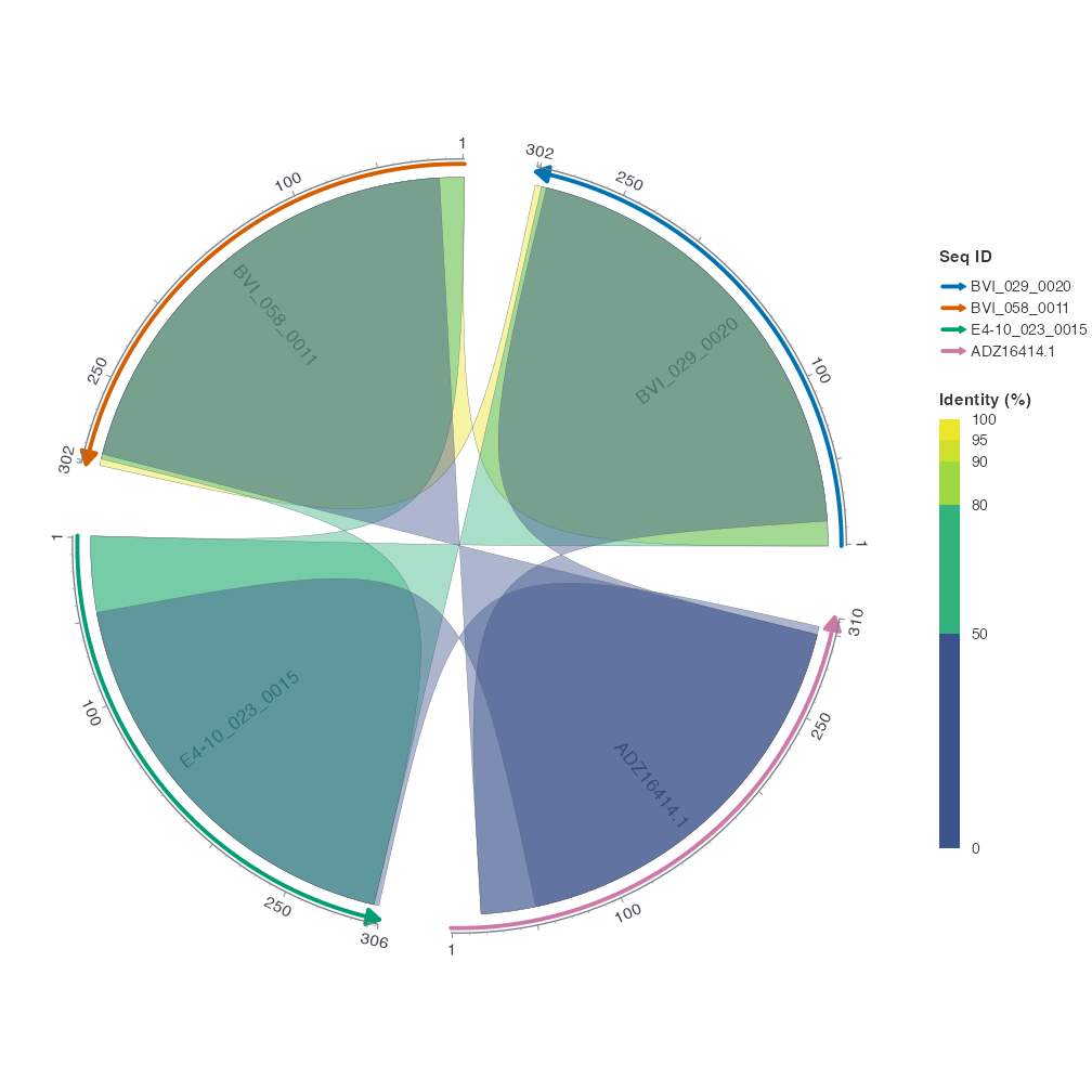
Pairwise identity ranges from about 35.7% to 99.0%. The plot uses the default Identity scale without additional colour settings.
Use generic layers such as geom_feature() for annotations at amino-acid positions, declaring directionality = "none" for nondirectional intervals. One plot uses either aa or bp. The endpoints of blastx and tblastn have different units and require conversion to one coordinate domain or separate displays. Gene arrows, primers and restriction sites require nucleotide input. A circular protein layout describes a visual arrangement.
2 Place protein hits on a nucleotide genome
To locate protein hits on a nucleotide backbone, provide known CDS mappings and project aa intervals into bp. This section uses source protein hits for BVI_023A_0009, selecting records with complete CDS before converting the query side. Inputs come directly from bundled sequence_detail_example; original provenance is available in the input bundle.
R · Example code
protein_source <- sequence_detail_example$protein_hits
emale_source <- sequence_detail_example$source_coding_features
# The source declares complete Prodigal CDS and translation table 11.
emale_coding <- emale_source |>
  filter(grepl("partial=00", attributes)) |>
  select(feature_id, accver, start, end, strand, phase)
emale_cds <- build_ggchord_cds(emale_coding, genetic_code = 11)
# Keep strong HSPs whose query protein has a known complete CDS.
# Gaps are retained: projecting one query span does not assert an ungapped pair.
protein_kept <- protein_source |>
  filter(qaccver %in% emale_coding$feature_id, evalue <= 1e-10, length >= 50) |>
  arrange(desc(bitscore))
selected_hsp <- protein_kept |>
  slice_head(n = 1)
select(selected_hsp, qaccver, qstart, qend, length, evalue)| qaccver | qstart | qend | length | evalue |
|---|---|---|---|---|
| BVI_023A_0009 | 50 | 289 | 250 | 7.19e-53 |
| accver | start | end | strand |
|---|---|---|---|
| BVI_023A | 7181 | 7900 | - |
| Metric | Observed output |
|---|---|
| Original BLASTp HSPs | 2948 |
| Complete query CDS records | 24 |
| Query HSPs retained by the explicit filter | 3 |
| Selected query start (aa) | 50 |
| Selected query end (aa) | 289 |
| Projected query-span rows | 1 |
Residues 50–289 project to 7,181–7,900 bp on BVI_023A, on the reverse strand. A single-end projection can retain the span of a gapped HSP. Connecting two genomes also requires the subject CDS model. See CDS projection for a supported ungapped two-ended example.
3 Data source
The bundled identifiers are BVI_029_0020, BVI_058_0011, E4-10_023_0015 and ADZ16414.1. Complete FASTA records come from public EMALE/Mavirus data. NCBI BLASTp 2.17.0+ computed all comparisons, retaining one HSP per pair. The raw output retains self hits and both directions, for 16 rows. The example table retains one direction per unordered pair in sequence-table order, without changing endpoints or identity.
The input bundle’s examples/protein/ directory retains complete FASTA records, raw BLASTp output and sources.json hashes. Rebuild rules are in data-raw/prepare-bundled-proteins.py and data-raw/generate_protein_data.R. Plotting uses bundled objects and does not require BLASTp.
4 Result checks
Check complete lengths, endpoints and units. Native protein plots use aa. Locating hits on a genome requires CDS projection to bp. Use view_ggchord() to inspect the target output size.