0.16.6 documentation

Site guide · find your task

Setup and learning paths

HomeInstall and prepare the environmentChoose your learning module

Module I · Chord

1.1 Tables and field meanings1.2 Produce and import comparisons1.3 Build the layers step by step1.4 Direction, curvature and clearance1.5 Filter and summarize links1.6 Full source-file workflow1.7 Complete chord showcase

Module II · Collinear

2.1 Reuse chord input tables2.2 Switch coordinates and add layers2.3 Routes, clearance and the ruler2.4 Compare CDS neighbourhoods2.5 Focus, anchors and segments2.6 Complete collinear showcase

Module III · Plasmid

3.1 DNA, annotations and 13 references3.2 From a circle to annotation layers3.3 Features, primers and restriction3.4 Thirteen plasmid references3.5 Complete plasmid cases

Consult as needed · Data and layers

Prepare tables and coordinatesImport and convert dataImport nucleotide and protein alignmentsProject protein intervals to genomic coordinatesFeatures, stacking and genomic decorationLabels and local placementQuantitative tracksMappings, scales, guides and themesSet values by sequence and strandCommon adjustments and grammarExport, preview and diagnostics

Learning map and reference

Articles and complete workflowsFunction referenceReproducible galleryFrequently asked questionsMigrate to the candidate APITerminology and design sourcesDevelopment status and changes

1.7 Complete chord showcase

On this page

• What this view shows
• Prepare original records
• Compose the layers
• Read and adapt the result
• Save at its intended size

Bring four genomes into one connected view. Combine straight and curved backbones, strand-aware genes and a continuous identity scale without hiding where the data came from.

What this view shows

Four-genome chord comparison with mixed backbone curvature and measured identity · Click to enlarge

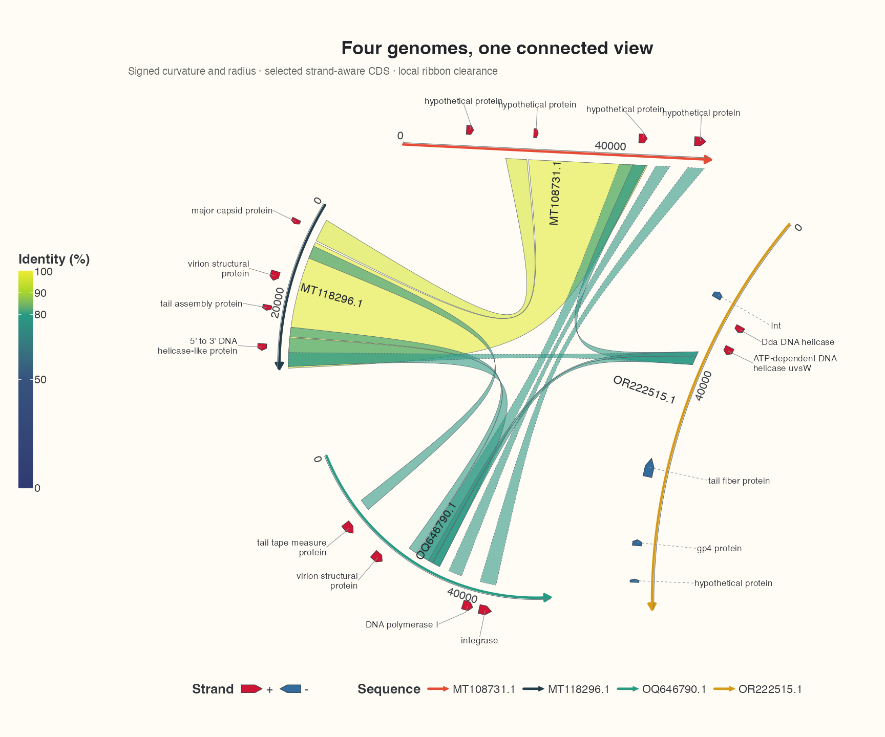
This is the end of Module I. Begin with tables, import, layer construction and geometry/clearance. 18 selected real CDS each receive repel labels; the complete 266-row annotation source remains separate. The four backbones combine zero, positive and negative curvature, varying radii and optimized display directions.

Prepare original records

Extract the tutorial input bundle into the working directory, so it contains examples/. Install the optional example packages with install.packages(c("dplyr", "purrr", "tidyr")); they prepare tables, map lists and inspect endpoint columns.

Preparation code — run once on this page

Code

# Optional appearance choices; none of these columns or scales is required input.
library(ggchord)
seq_palette <- setNames(
  c("#E64B35", "#233E4A", "#269B82", "#D59B17"),
  c("MT108731.1", "MT118296.1", "OQ646790.1", "OR222515.1")
)
gene_palette <- c("+" = "#CE1536", "-" = "#346B9D", "." = "#8291A6")

library(ggchord)
doc_background <- "#FFFCF5"
identity_palette <- c("#303B71", "#36537D", "#269B82", "#A5D52C", "#ECEB31")
identity_values <- c(0, 0.5, 0.8, 0.9, 1)
identity_breaks <- c(0, 50, 80, 90, 100)
doc_legend_theme <- theme(
  legend.title = element_text(size = 13, face = "bold"),
  legend.text = element_text(size = 11),
  legend.key.width = unit(9, "mm"), legend.key.height = unit(5, "mm"),
  legend.spacing.x = unit(9, "mm"), legend.spacing.y = unit(7, "mm"),
  legend.margin = margin(l = 4, r = 4, unit = "mm")
)
sequence_guide <- guide_ggchord_legend(nrow = 1, theme = doc_legend_theme)
strand_guide <- guide_ggchord_legend(
  nrow = 1, override.aes = list(strand = c("+", "-")), theme = doc_legend_theme
)
identity_guide <- guide_ggchord_colourbar(
  position = "left", direction = "vertical",
  theme = theme(
    legend.key.height = unit(75, "mm"), legend.key.width = unit(5, "mm"),
    legend.title = element_text(size = 13, face = "bold"),
    legend.text = element_text(size = 11), legend.margin = margin(r = 7, unit = "mm")
  )
)
doc_theme <- theme_ggchord_publication(
  axis.text = element_text(size = 11),
  axis.text.check.overlap = TRUE
) +
  theme(
    legend.position = "bottom",
    legend.title = element_text(size = 13, face = "bold"),
    legend.text = element_text(size = 11),
    legend.key.width = unit(9, "mm"), legend.key.height = unit(5, "mm"),
    legend.spacing.x = unit(9, "mm"), legend.spacing.y = unit(7, "mm"),
    legend.box.spacing = unit(6, "mm"),
    plot.background = element_rect(fill = doc_background, colour = NA),
    panel.background = element_blank(),
    plot.title = element_text(face = "bold", size = 18),
    plot.subtitle = element_text(size = 10, colour = "#5C625A"),
    plot.margin = margin(14, 18, 14, 18)
  )
doc_axis <- function(coordinates = "relative") {
  scale_seq_position_continuous(
    coordinates = coordinates, n.breaks = 3, minor_breaks = NULL,
    labels = function(x) format(x, scientific = FALSE, big.mark = ",", trim = TRUE)
  )
}

Code

library(ggchord)
library(dplyr)
library(purrr)
library(tidyr)
# Original repository records; extract the tutorial input bundle first.
show_sequences <- read_fasta_lengths(files = "examples/fasta/*.fna") |>
  select(accver, length)
show_annotations <- read_gff3(files = "examples/gff3/*.gff3", unstranded = "keep")
show_genes <- show_annotations |>
  filter(type == "CDS") |>
  select(accver, start, end, strand, anno)
show_alignments <- read_blast(files = "examples/blastn-standard/*.tsv")
# At most three substantial observed HSPs per pair; no coordinates are invented.
show_links <- show_alignments |>
  filter(length >= 900, pident >= 75) |>
  group_by(qaccver, saccver) |>
  slice_max(length, n = 3, with_ties = FALSE) |>
  ungroup()
# Select up to four source CDS per sequence, spread across annotation order.
# No feature is moved or invented; keep complete source tables separately.
show_features <- show_genes |>
  filter(end - start + 1 >= 500) |>
  group_by(accver) |>
  arrange(start, .by_group = TRUE) |>
  mutate(display_bin = ntile(row_number(), 4), informative = !is.na(anno) & anno != "hypothetical protein") |>
  group_by(accver, display_bin) |>
  arrange(desc(informative), desc(end - start), .by_group = TRUE) |>
  slice_head(n = 1) |>
  ungroup() |>
  select(accver, start, end, strand, anno)
# Also retain well-separated negative-strand CDS, if not already represented.
show_reverse <- show_genes |>
  filter(strand == "-", end - start + 1 >= 500) |>
  group_by(accver) |>
  arrange(start, .by_group = TRUE) |>
  slice(c(1, n())) |>
  ungroup()
show_features <- bind_rows(show_features, show_reverse) |>
  distinct(accver, start, end, strand, .keep_all = TRUE) |>
  arrange(accver, start)
show_labels <- show_features
show_optimization <- optimize_ggchord_layout(
  show_sequences, show_links,
  optimize = "orientation", weight = "length"
)

The input contains four unchanged FASTA records, their GFF3 annotations and 32 original HSPs. The display keeps HSPs at least 900 bp long and at least 75% identical, with at most three per sequence pair. This reduces clutter without merging or inventing alignments.

Compose the layers

Code

show_curvature <- c(
  "MT108731.1" = 0, "MT118296.1" = 0.85,
  "OQ646790.1" = 1.1, "OR222515.1" = -0.4
)
show_radius <- c(
  "MT108731.1" = 1, "MT118296.1" = 1.05,
  "OQ646790.1" = 0.95, "OR222515.1" = 1.08
)
p_show_chord <- ggchord(show_sequences, show_links, show_features) +
  geom_link_ribbon(aes(ribbon_fill = pident), link_avoid = "smooth", alpha = 0.58, linewidth = 0.18) +
  geom_seq(
    seq_orientation = show_optimization$seq_orientation,
    seq_curvature = show_curvature, seq_radius = show_radius,
    seq_gap = 0.06, linewidth = 1.1
  ) +
  geom_gene(position = position_strand(0.07), width = 0.035) +
  geom_gene_label_repel(
    data = show_labels, label_layout = "radial", label_wrap = 24,
    size = 3.1, label_max_lines = 3, position = position_strand(0.07)
  ) +
  geom_seq_label(size = 4, seq_label_radius = 0.84, seq_label_hjust = 0.5) +
  scale_seq_colour_manual(
    values = seq_palette, name = "Sequence",
    guide = sequence_guide
  ) +
  scale_gene_fill_manual(values = gene_palette, breaks = c("+", "-"), name = "Strand") +
  scale_ribbon_fill_gradientn(
    colours = identity_palette, values = identity_values,
    limits = c(0, 100), breaks = identity_breaks, name = "Identity (%)", guide = identity_guide
  ) +
  guides(gene_fill = strand_guide) +
  scale_seq_position_continuous(breaks = c(0, 20000, 40000), minor_breaks = NULL) +
  coord_chord(rotation = 50) +
  doc_theme +
  labs(
    title = "Four genomes, one connected view",
    subtitle = "Signed curvature and radius · selected strand-aware CDS · local ribbon clearance"
  )
p_show_chord

geom_seq(seq_curvature = ...) applies named values to stable sequence identifiers. 0 is a straight backbone. Curvature changes the display geometry; it does not alter sequence lengths, biological strands or alignment endpoints.

Read and adapt the result

Start with the sequence colours and gene directions, then trace the larger aligned intervals. A ribbon crossing is not evidence of a rearrangement by itself. The colour bar uses the same identity scale as the collinear view.

Use link filtering to change the display threshold, labels to choose annotation density, or sequence parameters to change radius and curvature. For a file-by-file introduction, start with original sequence comparisons.

Save at its intended size

Code

ggsave("four-genome-chord.png", p_show_chord, width = 12, height = 10, units = "in", dpi = 144)