Chapters and reference
Shared techniques · Section 3 of 10
5.2 Gene and feature arrow geometry
On this page
Compare arrow outlines on the same observed CDS. Choose shape before size; neither changes the interval, strand or biological function.
1 Prepare a real annotation and local window
Use the bundled integrase in gene_data_example: OQ646790.1 at 43,765–46,140 bp. Restore the original positive strand from source_strand. Focus on 43,000–47,000 bp for visibility and display source coordinates on the axis.
R · Example code
library(ggchord)
library(dplyr)
source_gene <- gene_data_example |>
  filter(accver == "OQ646790.1", start == 43765) |>
  transmute(accver, start, end, strand = source_strand, anno)
gene_window <- focus_ggchord_data(
  seq_data = filter(seq_data_example, accver == "OQ646790.1"),
  gene_data = source_gene,
  loci = data.frame(accver = "OQ646790.1", start = 43000, end = 47000)
)
gene_base <- ggchord(gene_window$seq_data, gene_data = gene_window$gene_data) +
  geom_seq() +
  scale_seq_position_continuous(coordinates = "source") +
  coord_collinear()
gene_window retains clipping and source metadata. Your CDS needs a complete sequence length, matching accver, one-based inclusive start/end, and an evidence-backed strand. Use geom_feature() for unknown strands. This page runs independently in a new R session and requires the optional dplyr package.
2 Select the real neighbourhood by explicit ID
Combine source accession/endpoints into a workflow target ID, not a claimed database gene ID. Find_ggchord_loci selects exact IDs and extends 100 bp upstream/downstream in biological direction. Negative-strand upstream points to larger source coordinates; unknown/bidirectional strands require symmetric extensions. Pass returned windows to focus_ggchord_data and inspect full-length boundary clipping flags.
Output / text
               target_id               locus_id     accver start   end strand target_start target_end upstream downstream clipped_left clipped_right target_source_rows
1 OQ646790.1:43765:46140 OQ646790.1:43765:46140 OQ646790.1 43665 46240      +        43765      46140      100        100        FALSE         FALSE                  1
3 Three arrow constructions
All figures use 9 × 4 inches and identical input, window and layers. To expose shoulders, all three explicitly use arrow_head_width = 1.6 (default 1). Only arrow_head_style changes.
R · Example code
p_comparegeneshouldered <- gene_base + geom_gene(arrow_head_width = 1.6, arrow_head_style = "shouldered")
view_ggchord(p_comparegeneshouldered, width = 9, height = 4, units = "in")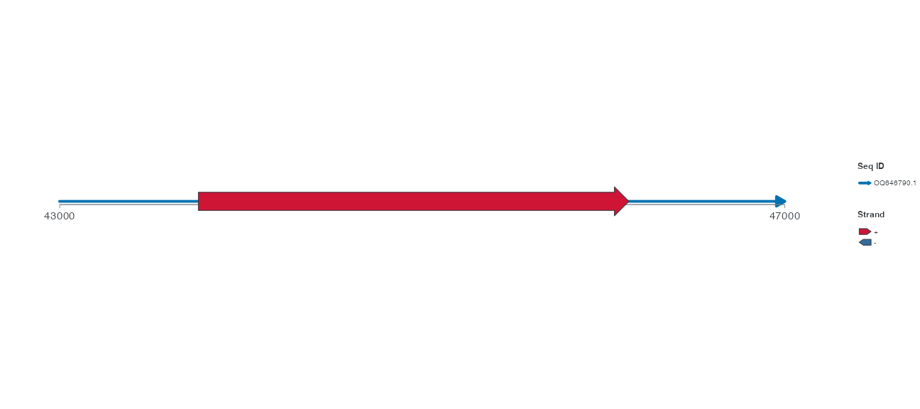
shouldered is the default construction. A wider head creates shoulders where it joins the shaft, emphasizing direction.
R · Example code
p_comparegeneflush <- gene_base + geom_gene(arrow_head_width = 1.6, arrow_head_style = "flush")
view_ggchord(p_comparegeneflush, width = 9, height = 4, units = "in")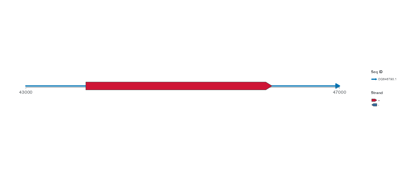
flush uses a flush head-to-shaft outline. Compare the head junction while keeping the same endpoints and shaft.
R · Example code
p_comparegenetriangle <- gene_base + geom_gene(arrow_head_width = 1.6, arrow_head_style = "triangle")
view_ggchord(p_comparegenetriangle, width = 9, height = 4, units = "in")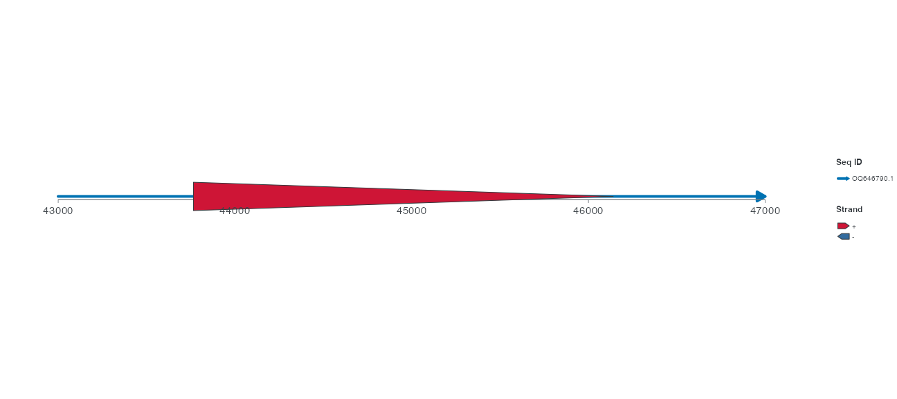
triangle draws the entire interval as a triangular wedge rather than adding a head to a rectangular shaft. Shape differences do not imply different functions or measured values.
4 When a short feature cannot fit its head
Keep the same observed integrase and window, requesting head length 1.5 in all three plots so the interval is short relative to its head. Change only short_feature: auto chooses a compressed directional glyph, wedge a wedge, block an undirected block. Do not lengthen source coordinates to fit a head; a block does not make the biological strand unknown.
R · Example code
p_compareshortauto <- gene_base + geom_gene(arrow_head_length = 1.5, short_feature = "auto")
view_ggchord(p_compareshortauto, width = 9, height = 4, units = "in")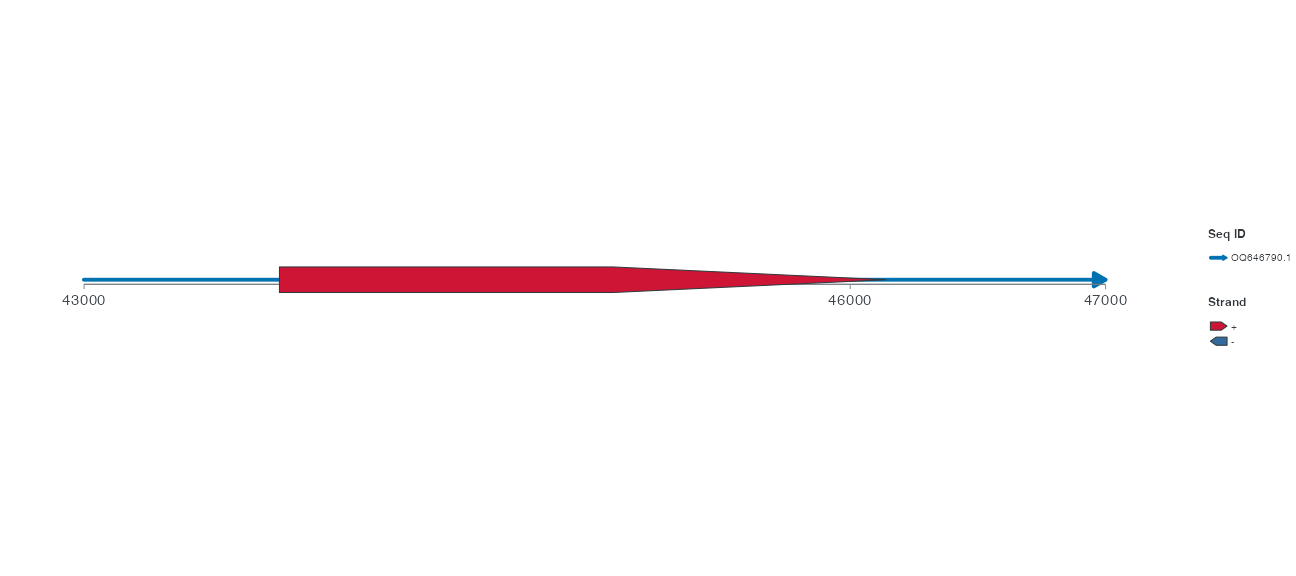
R · Example code
p_compareshortwedge <- gene_base + geom_gene(arrow_head_length = 1.5, short_feature = "wedge")
view_ggchord(p_compareshortwedge, width = 9, height = 4, units = "in")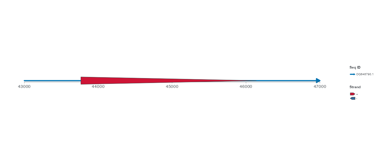
R · Example code
p_compareshortblock <- gene_base + geom_gene(arrow_head_length = 1.5, short_feature = "block")
view_ggchord(p_compareshortblock, width = 9, height = 4, units = "in")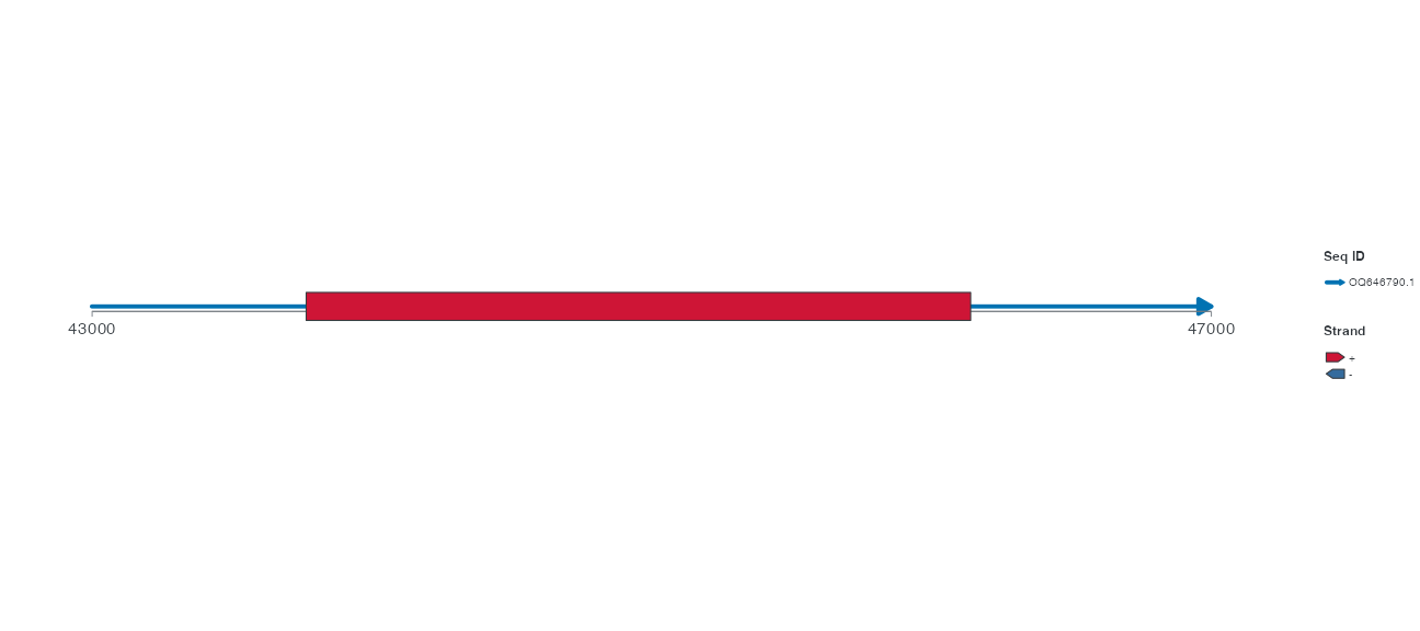
5 Dimensions, short features and presets
| Parameter |
geom_gene() default |
Values and choices |
|---|---|---|
width |
NULL, resolving to 0.05 |
Shaft width; may vary by sequence or strand |
arrow_head_length |
0.04 |
Head length in the local frame, not bp |
arrow_head_width |
1 |
Head width relative to the shaft; 1.6 in all three figures |
arrow_head_style |
"shouldered" |
shouldered / flush / triangle |
short_feature |
"auto" |
Selects wedge or block when the head cannot fit; explicit wedge/block fixes the fallback |
position |
"identity" |
position_strand separates strands; position_feature_stack separates overlaps |
Do not hide short intervals by enlarging heads. Check source length before choosing a fallback. Generic geom_feature() accepts fixed shape or mapped aes(feature_shape = ...) with a corresponding scale; see styling.
geom_feature_plasmid() is a preset with different width, head dimensions and Position defaults. Changing several defaults while comparing it to gene is not a single-parameter experiment. Segmented annotation boundaries mark segments, not different genes.
6 Modes, input adaptation and next steps
Gene arrows support bp inputs in chord, collinear and single circular modes. Use generic features for aa intervals. Focusing and display reversal do not rewrite biological strand; see compatibility.
First change the common head width from 1.6 back to 1 and inspect shoulder visibility. Then change only width and compare shaft versus backbone width. Keep export dimensions fixed rather than editing source intervals to improve appearance.
Continue with feature stacking, labels, or add this CDS to the four-genome example. Full interfaces: geom_gene(), geom_feature().