Chapters and reference
Module I · Multi-sequence relationships · Section 11 of 16
1.10 Collinear: alignment and ordering
On this page
Data preparation and settings (expand)
R · Example code
chord_links <- head(ribbon_data_example, 1)Start with your first collinear plot, then compare alignment, anchors and orientation on the same real input. No chord sections are required.
1 Input and default left alignment
This page independently loads four bundled complete sequences and their observed alignments. Sequences need accver`, `length; links need both IDs and query/subject endpoints in bp, one-based inclusive. Preserve reverse endpoints rather than sorting them.
R · Example code
library(ggchord)
seqs_align <- seq_data_example[c("accver", "length")]
links_align <- ribbon_data_example[c("qaccver", "saccver", "qstart", "qend", "sstart", "send")]
base_align <- ggchord(seqs_align, ribbon_data = links_align) +
  geom_seq() +
  geom_link_ribbon() +
  geom_seq_label()
p_alignleft <- base_align + coord_collinear(align = "left")
view_ggchord(p_alignleft, width = 9, height = 6, units = "in")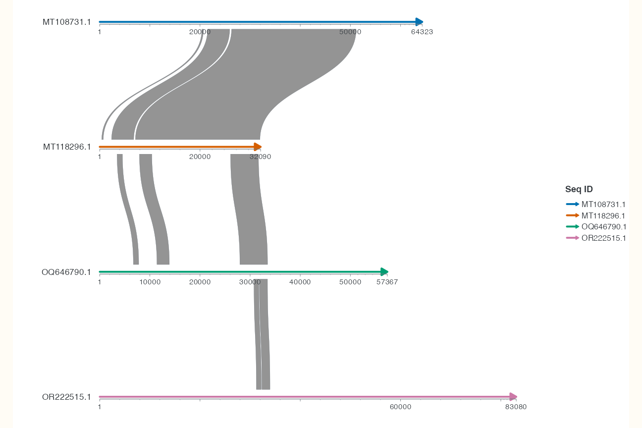
base_align keeps the data and layers fixed. Only coordinates change below. Defaults are align = "left", anchor = NULL, and orientation = "manual". All backbones share one horizontal scale; short sequences are not stretched.
2 Change alignment alone
R · Example code
p_aligncenter <- base_align + coord_collinear(align = "center")
view_ggchord(p_aligncenter, width = 9, height = 6, units = "in")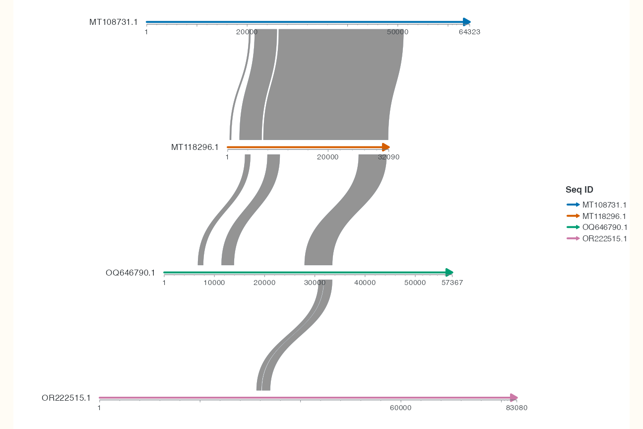
The complete sequence midpoints align. Each sequence translates independently, while its link positions on the backbone remain unchanged.
R · Example code
p_alignright <- base_align + coord_collinear(align = "right")
view_ggchord(p_alignright, width = 9, height = 6, units = "in")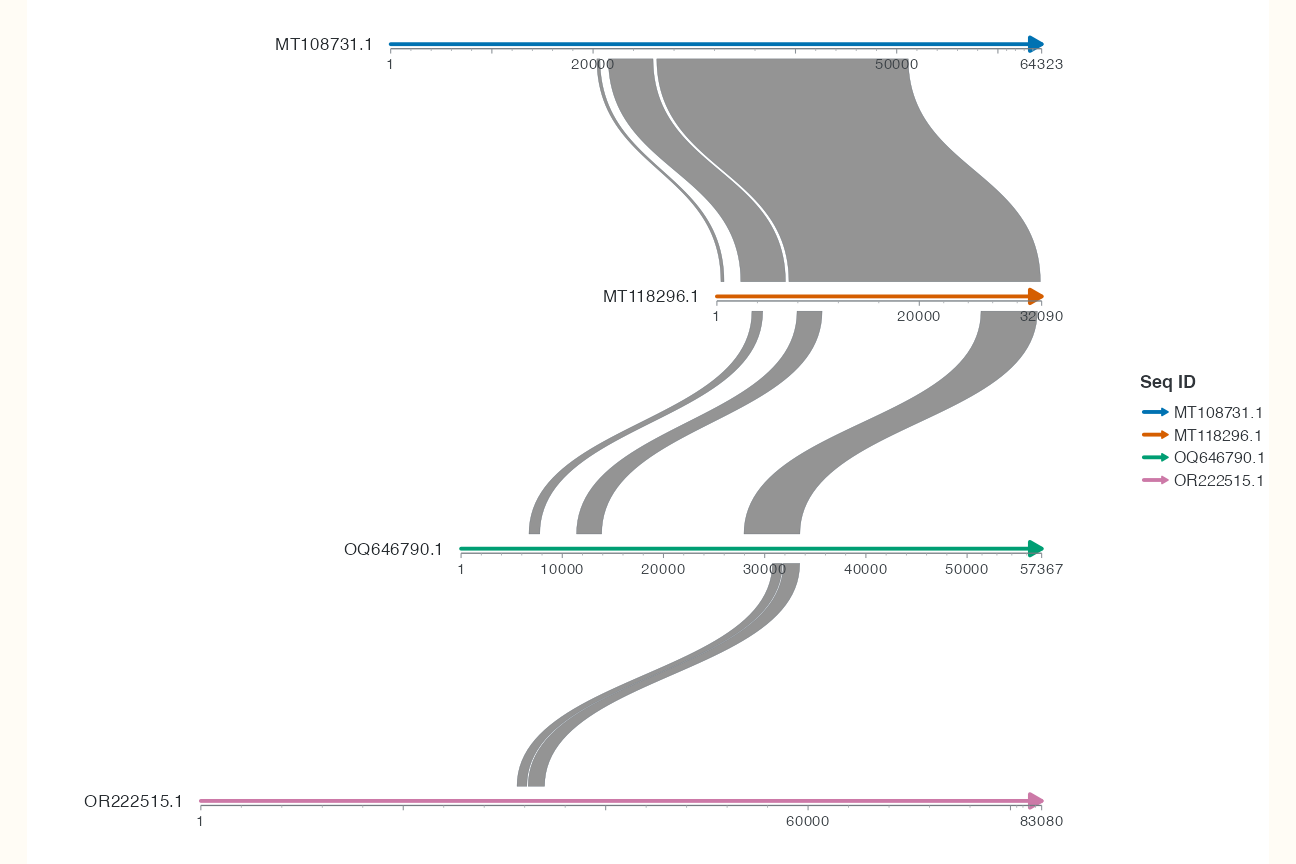
Right edges align. All three figures use 9 × 6 inches, identical data, layers, row order and directions. This compares translation, not newly computed alignments.
3 Supply one anchor per sequence
R · Example code
anchors <- setNames(seqs_align$length / 2, seqs_align$accver)
p_alignanchor <- base_align + coord_collinear(align = "left", anchor = anchors)
view_ggchord(p_alignanchor, width = 9, height = 6, units = "in")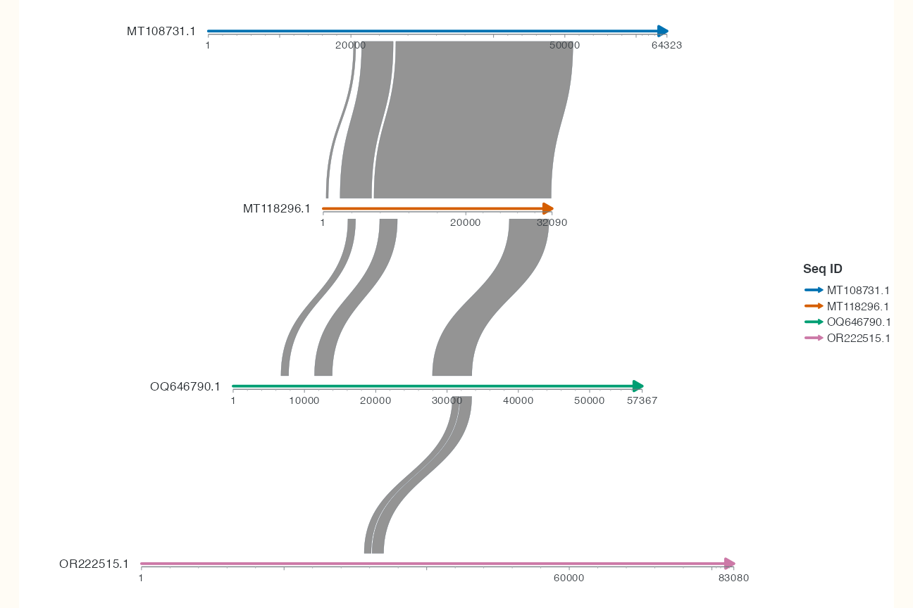
Relative to the left-aligned baseline, only anchor is added. The vector uses accver names and source sequence midpoints, so this example has the same effect as centering complete sequences. These are geometric demonstration anchors. Research anchors should come from explicitly justified common loci.
Alternatively supply a table with accver, position or accver, start, end. Every displayed sequence needs exactly one anchor; missing or duplicate anchors are errors. For intervals, align selects the displayed left edge, midpoint or right edge after orientation. Select a specific copy before anchoring multicopy genes.
4 Choose display directions automatically
R · Example code
p_alignauto <- base_align + coord_collinear(orientation = "auto", min_support = 0.1)
view_ggchord(p_alignauto, width = 9, height = 6, units = "in")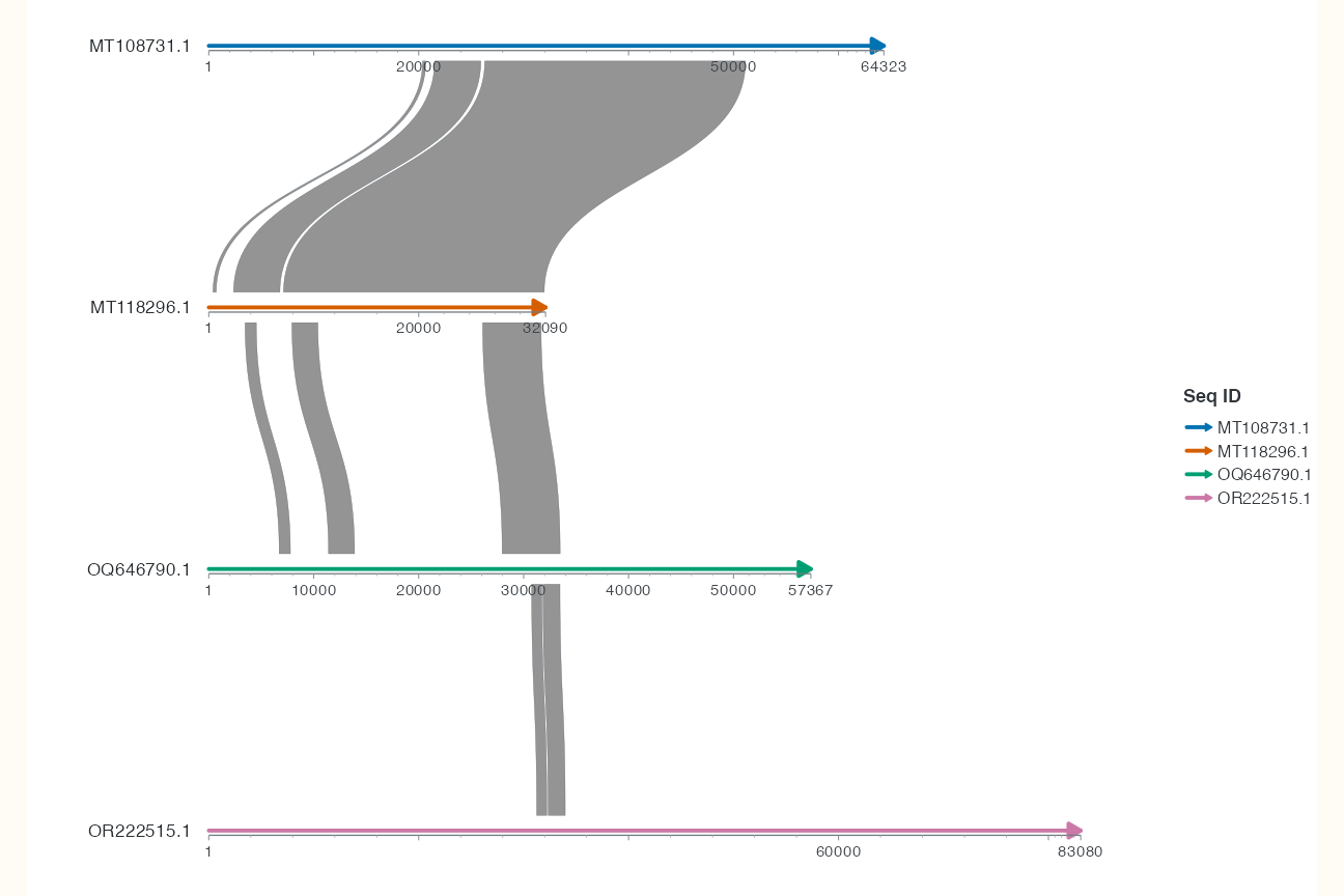
Only orientation = "auto" changes from the left-aligned baseline; min_support = 0.1 explicitly restates its default. The heuristic uses existing links to earlier displayed sequences; the first sequence fixes the reference. The threshold is the absolute forward/reverse support difference divided by their total, between 0 and 1. Ties, insufficient support and disconnected sequences retain their initial direction. An unchanged plot can mean that the evidence supports the initial directions, rather than that auto was ignored. Inspect diagnostics from export_ggchord_layout() rather than judging correctness by visual neatness.
| Concept | Data or setting | Meaning |
|---|---|---|
| Source sequence direction | FASTA record order | Reference for input coordinates |
| Biological gene strand | Annotation strand
|
Transcription direction relative to the source |
| Alignment direction | Increasing or decreasing endpoints | Relative match direction between intervals |
| Display direction |
seq_orientation or automatic orientation |
Placement in the plot |
A display flip does not rewrite source strands or establish a biological inversion. Do not combine explicit geom_seq(seq_orientation = ...) with automatic orientation.
5 Parameters and combination boundaries
| Parameter | Default | Type, effect and constraints |
|---|---|---|
align |
"left" |
left/center/right; aligns complete sequences or anchors |
anchor |
NULL |
Named numeric vector or table; does not crop data |
orientation |
"manual" |
manual/auto; auto conflicts with explicit sequence directions |
min_support |
0.1 |
Number in 0–1; directional evidence threshold, not identity |
segments |
NULL |
Explicit window table; conflicts with anchor or auto |
segment_gap |
100 |
Positive display distance in bp scale units, not omitted length |
These belong to coord_collinear(), not the other coordinate systems. Window tables own orientation in segmented views. Circular radius and curvature settings cannot be converted to this mode.
6 Use your own data
First change only align from left to right and observe short sequences against the longest backbone. Then choose a justified anchor for each sequence and explain why they can be compared. For your FASTA lengths and BLAST/PAF endpoints, check IDs, units, complete lengths and reverse endpoints; see data import.
For missing links inspect endpoints and adjacent-row filtering in cross-row connections. Continue with local windows and segments; see coord_collinear() for the complete reference.
7 Increase row spacing
R · Example code
p_linear_gap <- ggchord(seq_data = seq_data_example) +
  geom_seq(seq_gap = c("MT108731.1" = 0.45)) +
  geom_seq_label() +
  coord_collinear() +
  geom_link_ribbon(data = chord_links)
view_ggchord(p_linear_gap, width = 8, height = 5, units = "in")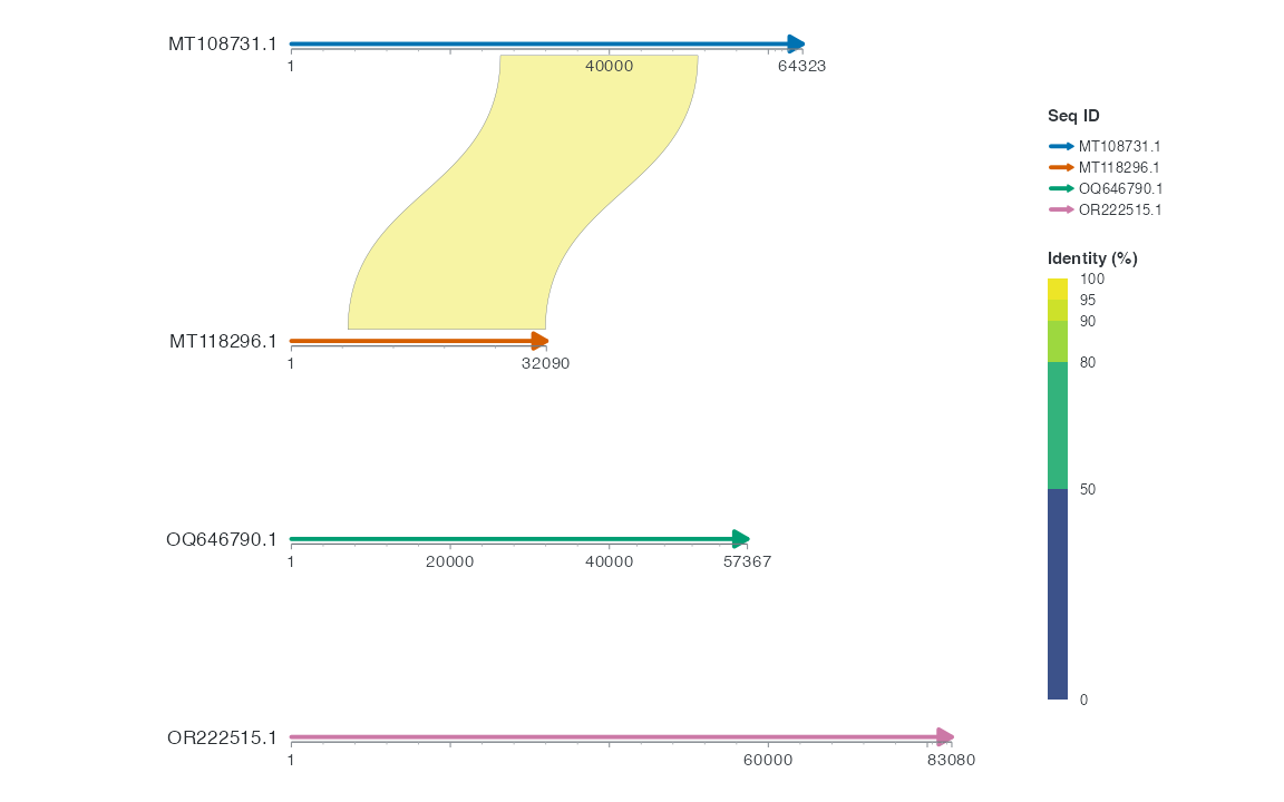
In a collinear plot, seq_gap is relative to the longest backbone width and defaults to 0.30. Set the gap below MT108731.1 to 0.45. The other gaps retain 0.30; the final row has no following gap. The ribbon still joins the same bp intervals.