Site guide · find your task
Reproducible gallery
On this page
- Find a figure by task
- Figures and dimensions
- Bundled sequences and alignment intervals in a chord view
- pUC19 annotations in a circular map
- Bundled records aligned to explicitly selected annotation anchors
- GC fractions computed from the bundled pUC19 DNA
- Focused sequence windows with source-coordinate axes
- Automatic placement of informative source gene annotations
- Original sequences with explicitly selected CDS and alignment links
- Original sequences, all imported CDS and filtered links
- pUC19 features, exact primer hits and three selected restriction sites
- Interval density from the original alignment observations
- Midpoint links derived from existing HSP intervals
- Stacked overlapping annotations from the pUC19 reference
- pUC19 GC fractions, a three-bin moving mean and annotation bands
- AmpR neighbourhoods: identical CDS, 200 bp flanks and source coordinates
- Highlighting the query interval of an observed alignment
- Informative gene annotations with automatic side placement
- The same gene annotations with radial placement
- The same gene annotations with arc-oriented text
- Explicit sequence, strand and query-category colour scales
- A real minimap2 PAF comparison between two EMALE genomes
- Your first plot: two bundled sequences, gene arrows and observed alignment intervals
- Four-genome chord comparison with mixed backbone curvature and measured identity
- Dense pETDuet-1 map: features, reference primers and grouped restriction sites
- Four-genome collinearity: strand-separated features and routed cross-row links
- Chord step1: sequence backbones
- Chord step2: observed comparisons
- Chord step3: selected genes
- Chord step4: labels for selected features
- The same backbones with linear coordinates
- The same observed links with linear coordinates
- The same genes and labels with linear coordinates
- pUC19 step1: double backbone
- pUC19 step2: features
- pUC19 step3: labels
- pSB1C3: source-backed feature map
- pUC19: source-backed feature map
- pBR322: source-backed feature map
- pBluescript II SK(+): source-backed feature map
- pET-28a(+): source-backed feature map
- pETDuet-1: source-backed feature map
- pDONR221: source-backed feature map
- pcDNA3.1(+): source-backed feature map
- pTRE-Tight-BI: source-backed feature map
- pTRIPZ: source-backed feature map
- pCAMBIA1300: source-backed feature map
- pEarleyGate 201: source-backed feature map
- pSpCas9(BB)-2A-GFP (PX458): source-backed feature map
- One source for both languages
- Reproduce
- Asset sources
Choose an example by the question it answers. Thumbnails help you navigate; click for full size. Every figure links to preparation, code and interpretation.
Find a figure by task
| Overall relationships | One annotated sequence | Local positions | Quantities and text |
|---|---|---|---|
| Chord | Plasmid | CDS neighbourhood | GC tracks |
| Point links | Feature stacking | Focus | Label layouts |
Figures and dimensions
Bundled sequences and alignment intervals in a chord view
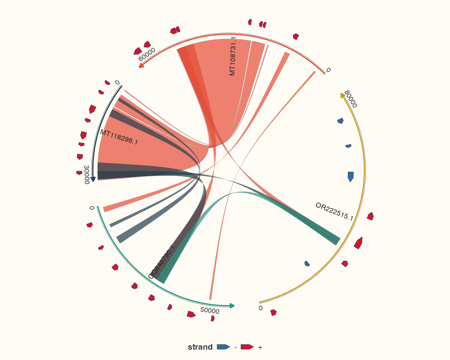
Data, code and interpretation →
p_chord · 10 × 8 in · 144 dpi
pUC19 annotations in a circular map
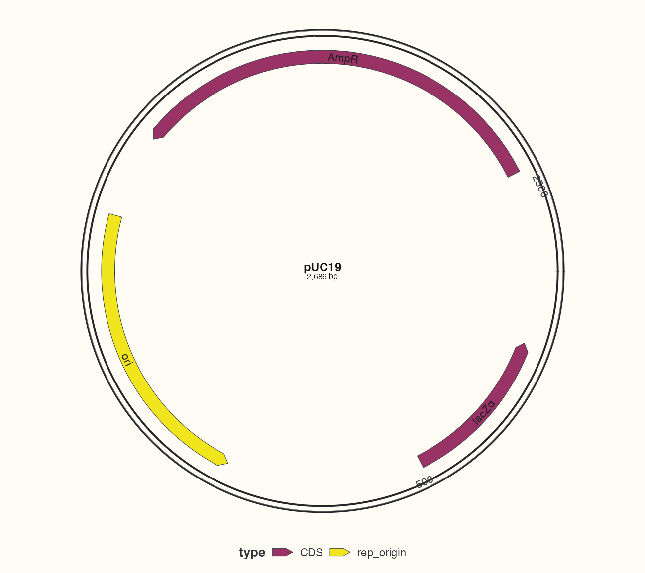
Data, code and interpretation →
p_circular · 9 × 8 in · 144 dpi
Bundled records aligned to explicitly selected annotation anchors
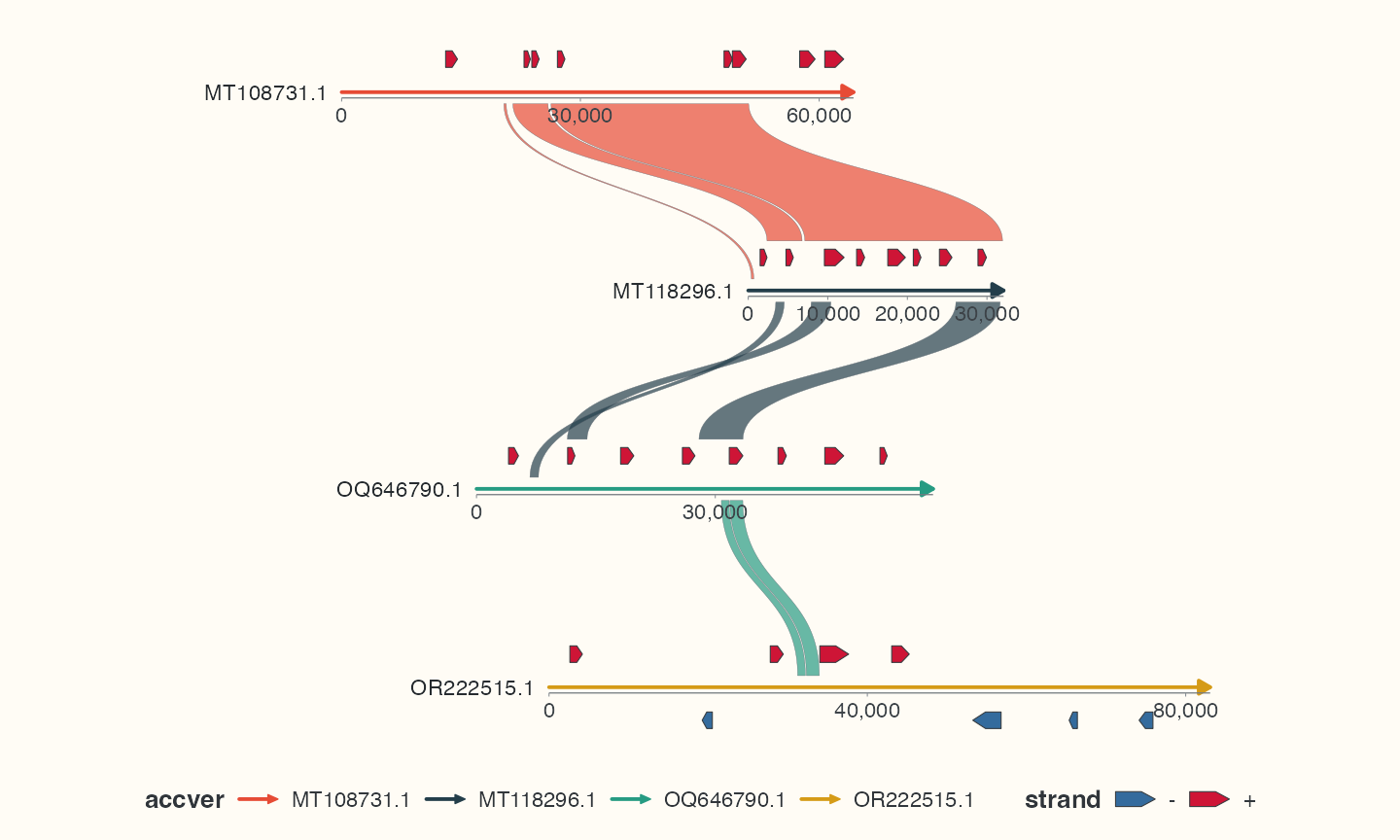
Data, code and interpretation →
p_collinear · 10 × 6 in · 144 dpi
GC fractions computed from the bundled pUC19 DNA
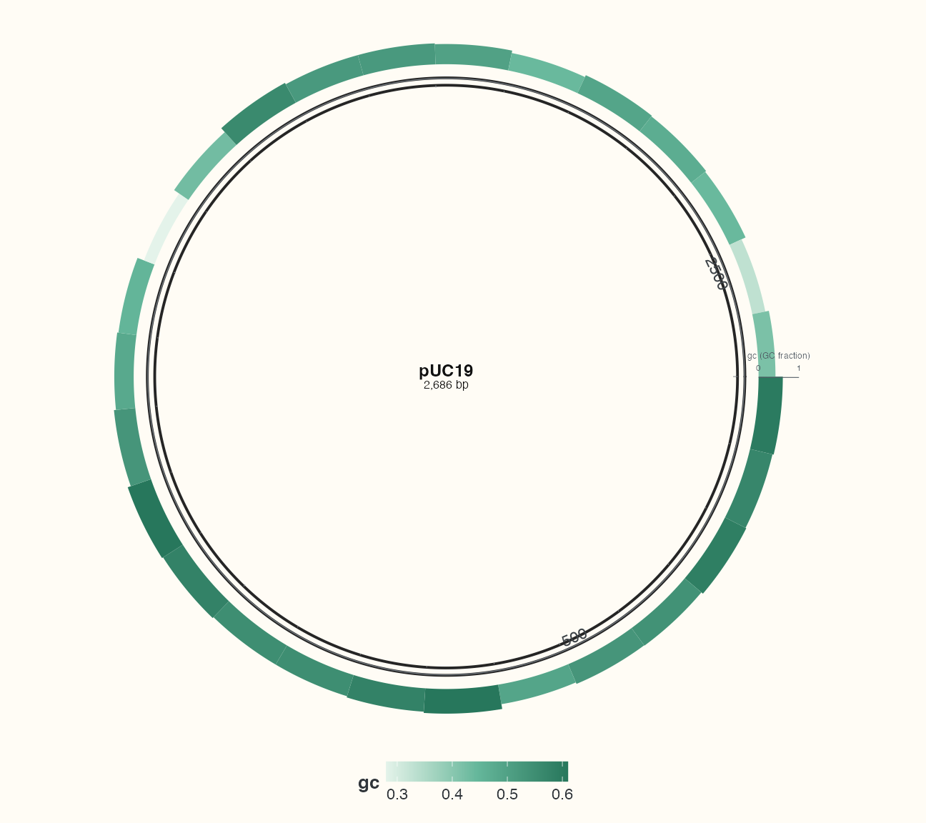
Data, code and interpretation →
p_tracks · 9 × 8 in · 144 dpi
Focused sequence windows with source-coordinate axes
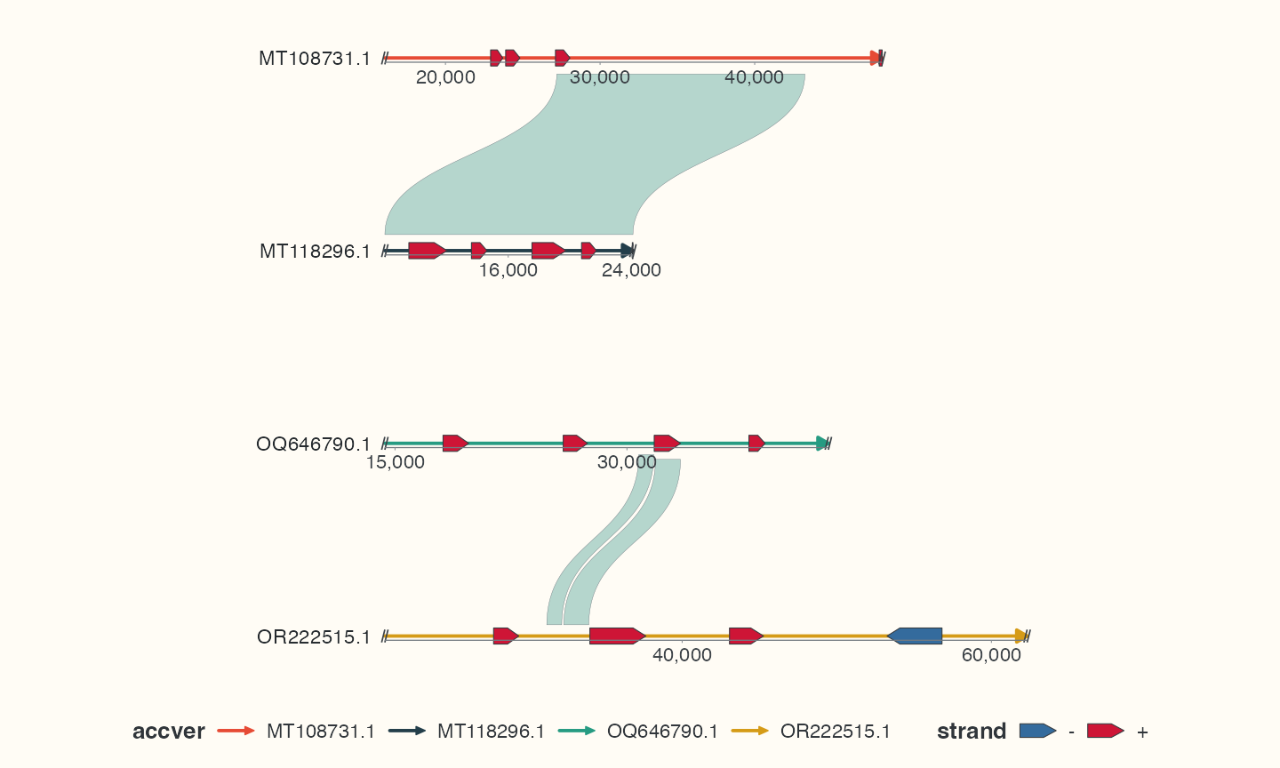
Data, code and interpretation →
p_focus · 10 × 6 in · 144 dpi
Automatic placement of informative source gene annotations
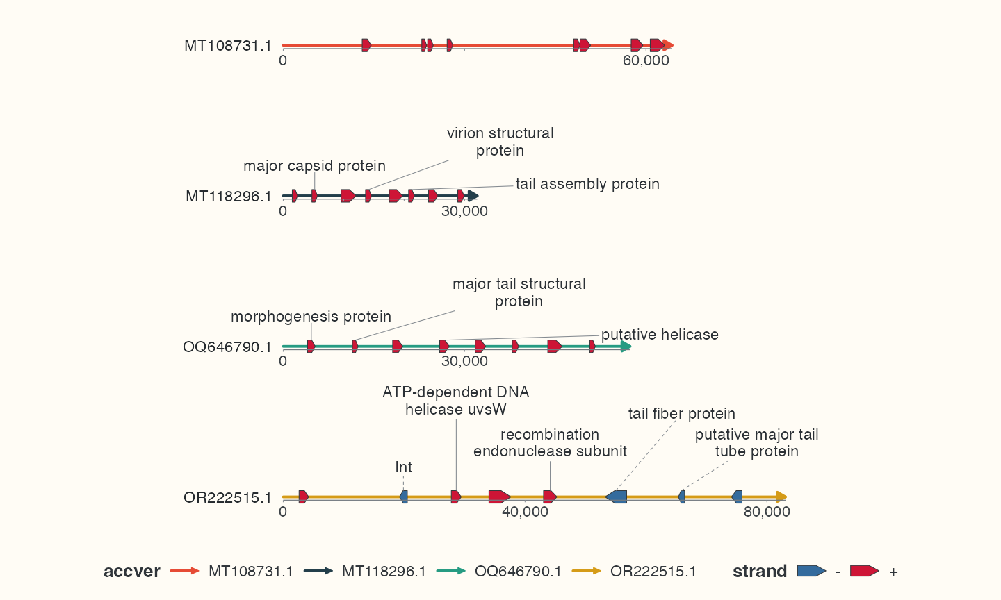
Data, code and interpretation →
p_labels · 10 × 6 in · 144 dpi
Original sequences with explicitly selected CDS and alignment links
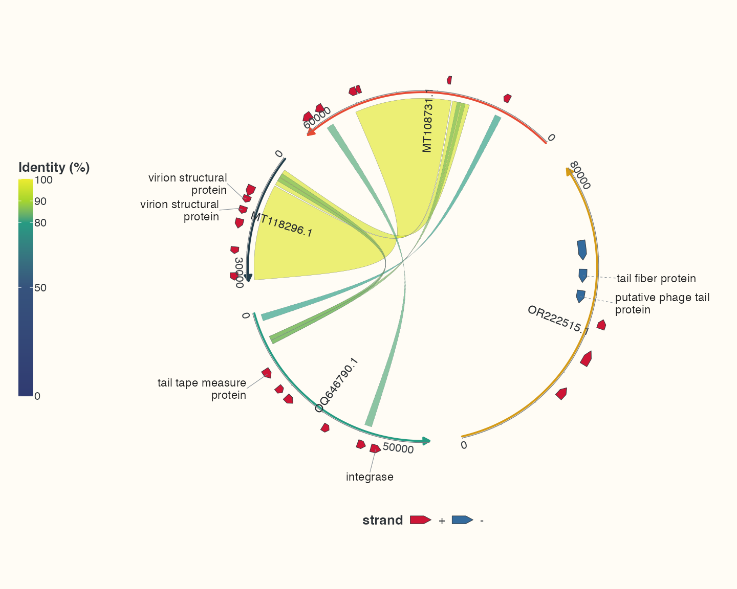
Data, code and interpretation →
p_real_chord · 10 × 8 in · 144 dpi
Original sequences, all imported CDS and filtered links
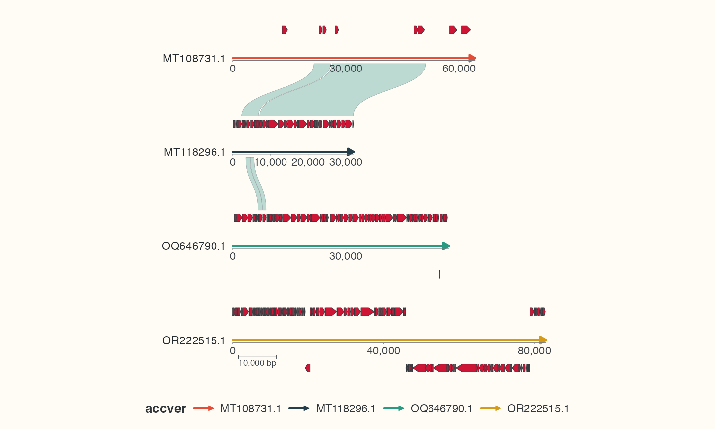
Data, code and interpretation →
p_real_linear · 10 × 6 in · 144 dpi
pUC19 features, exact primer hits and three selected restriction sites
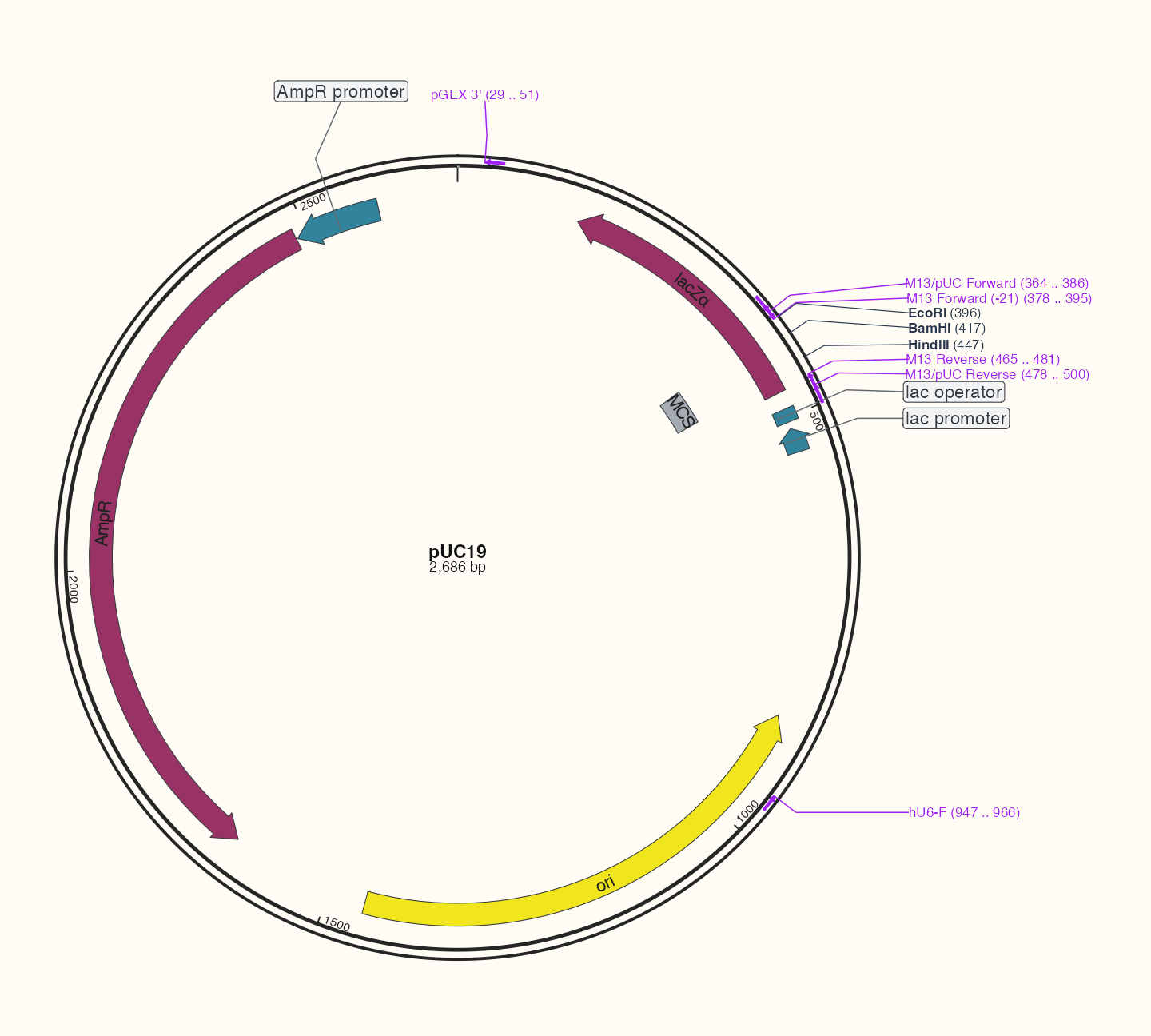
Data, code and interpretation →
p_plasmid · 10 × 9 in · 144 dpi
Interval density from the original alignment observations
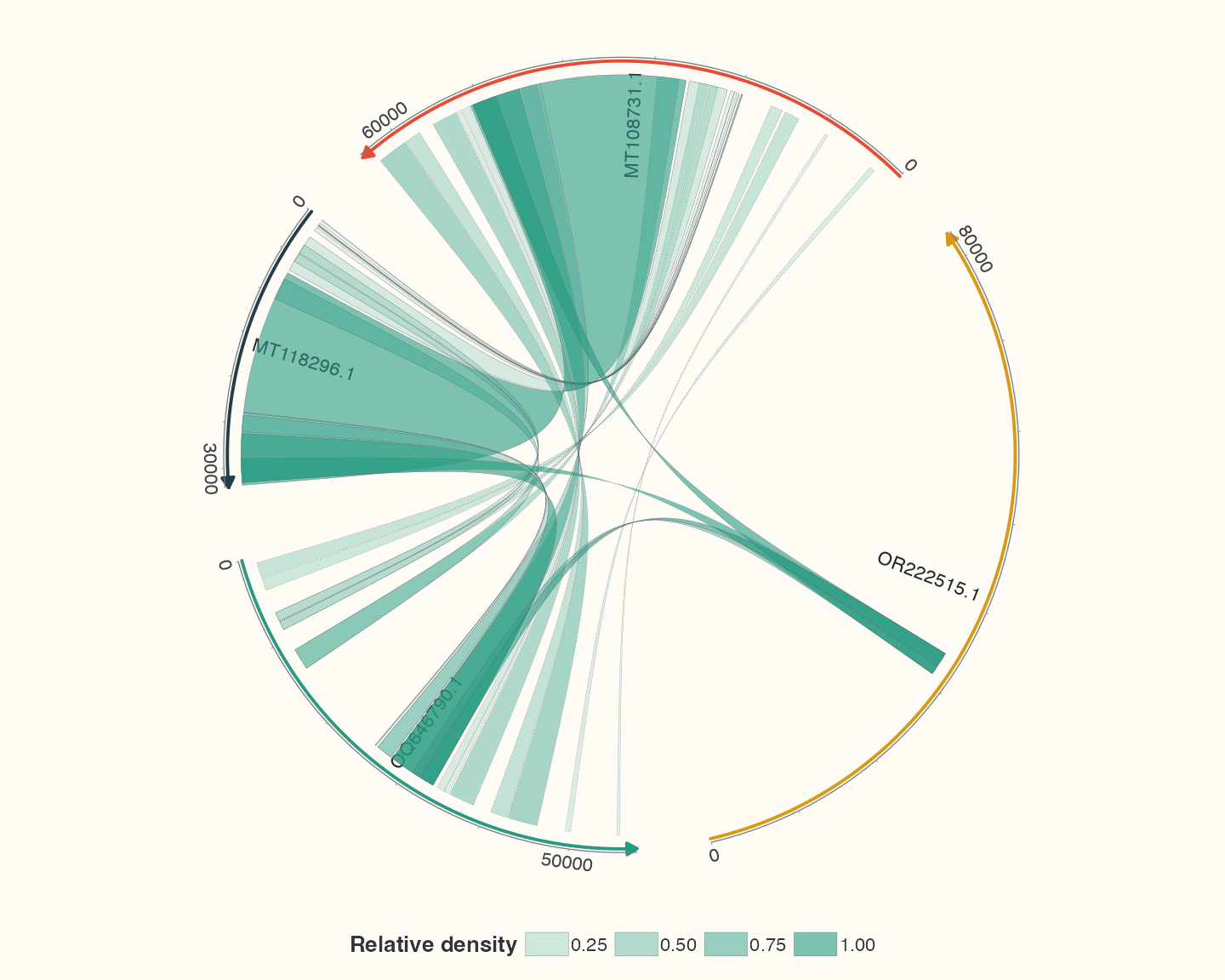
Data, code and interpretation →
p_density · 10 × 8 in · 144 dpi
Midpoint links derived from existing HSP intervals
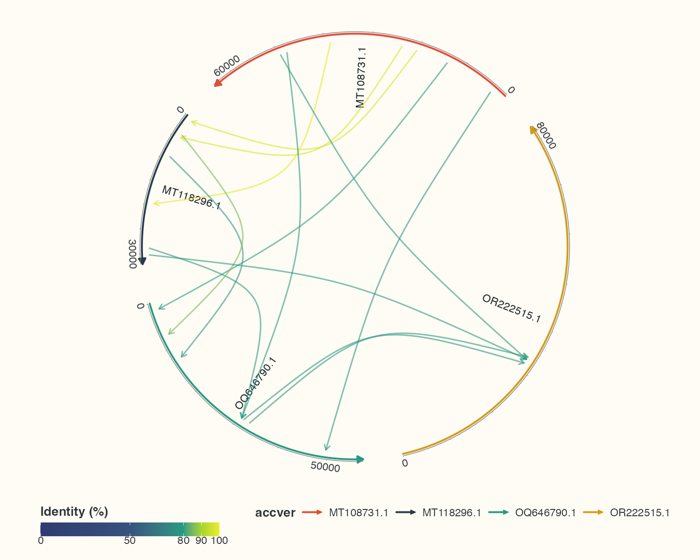
Data, code and interpretation →
p_points · 10 × 8 in · 144 dpi
Stacked overlapping annotations from the pUC19 reference
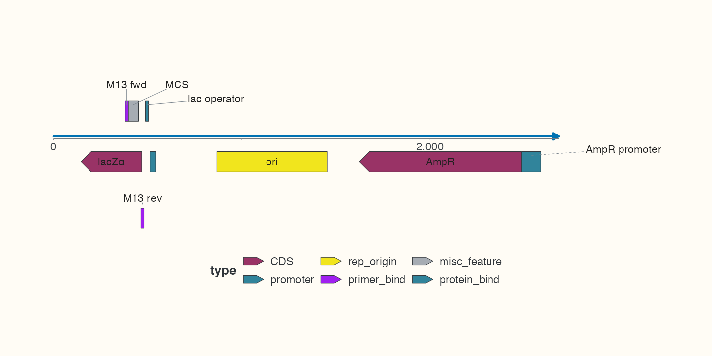
Data, code and interpretation →
p_stack · 10 × 5 in · 144 dpi
pUC19 GC fractions, a three-bin moving mean and annotation bands
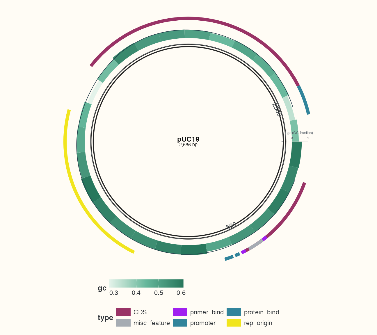
Data, code and interpretation →
p_multitrack · 9 × 8 in · 144 dpi
AmpR neighbourhoods: identical CDS, 200 bp flanks and source coordinates
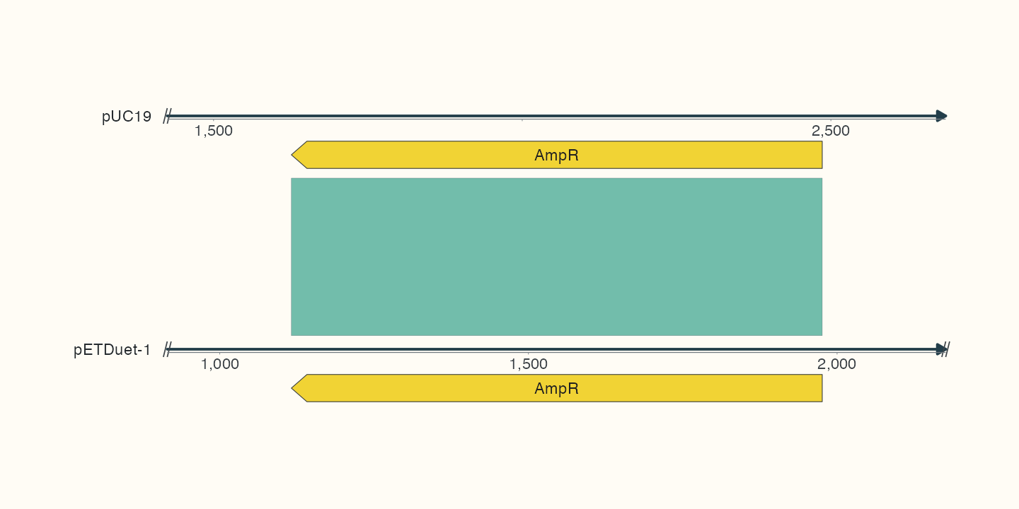
Data, code and interpretation →
p_homologs · 10 × 5 in · 144 dpi
Highlighting the query interval of an observed alignment
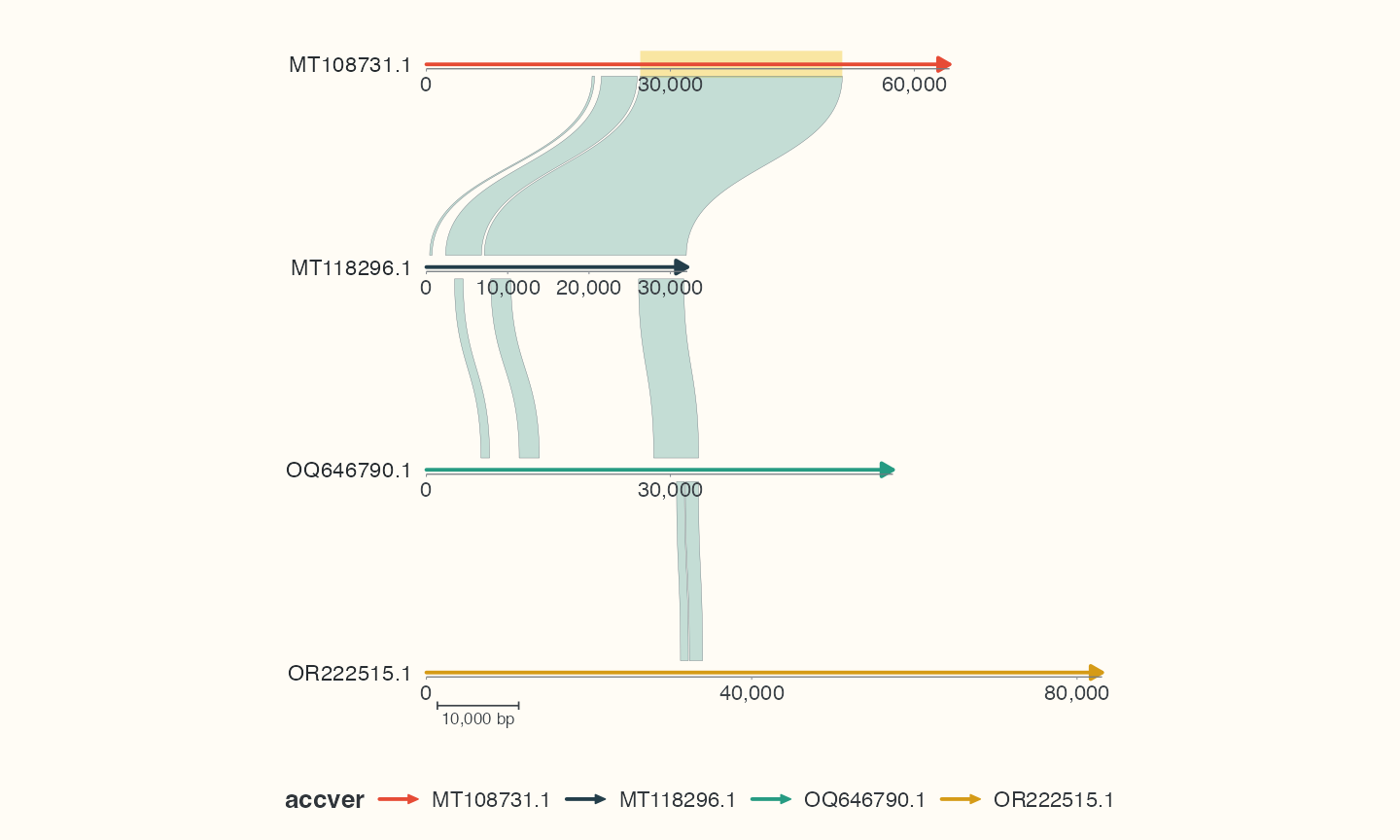
Data, code and interpretation →
p_decorated · 10 × 6 in · 144 dpi
Informative gene annotations with automatic side placement
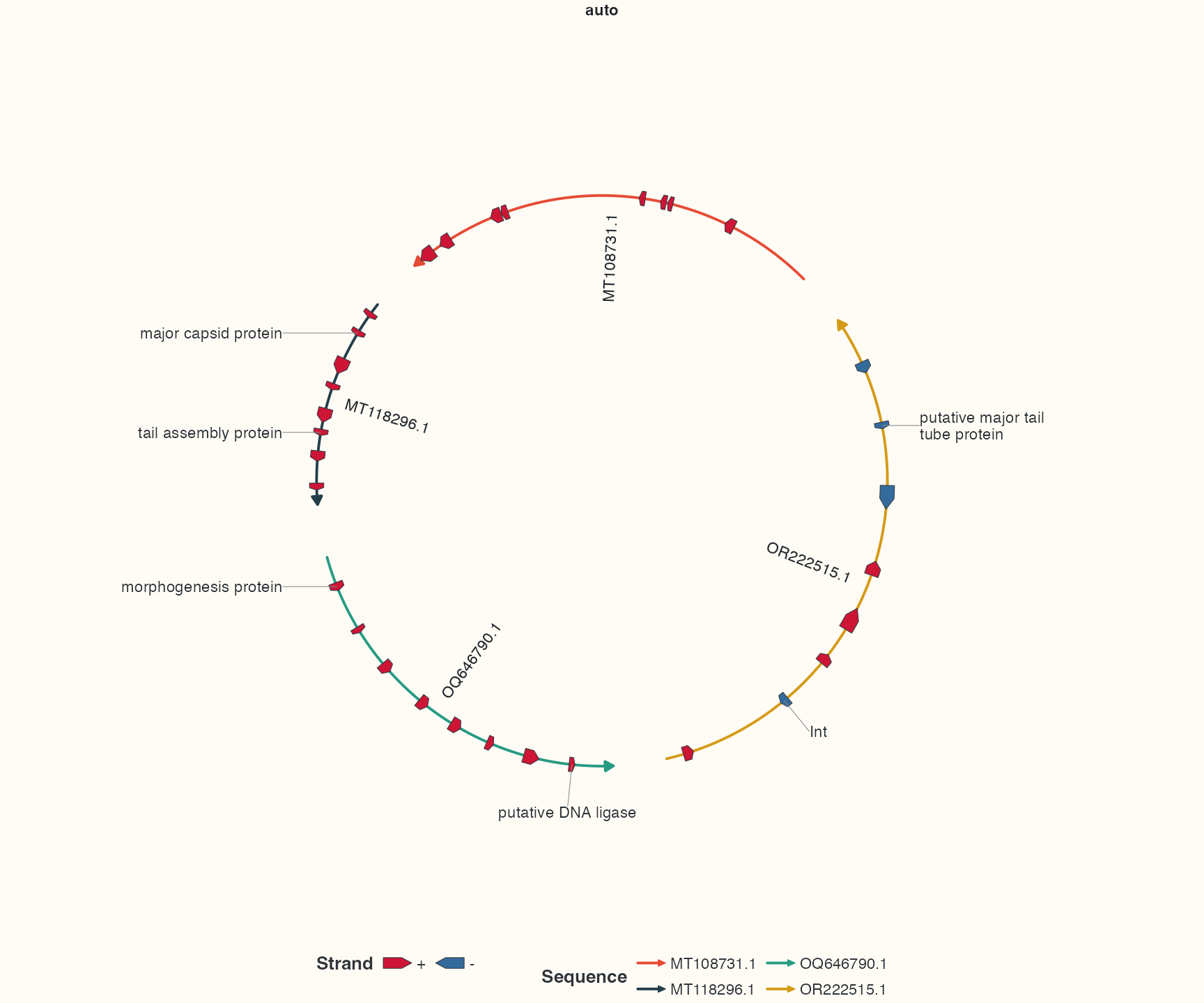
Data, code and interpretation →
p_labelauto · 12 × 10 in · 144 dpi
The same gene annotations with radial placement
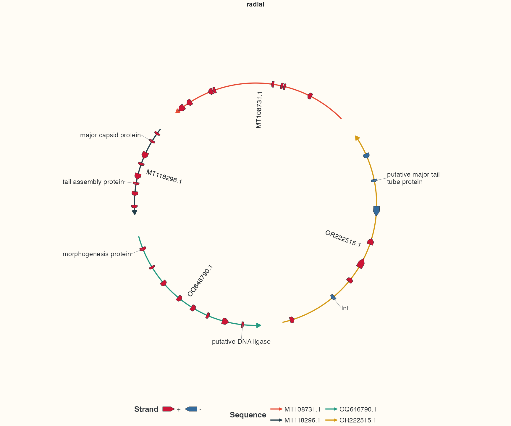
Data, code and interpretation →
p_labelradial · 12 × 10 in · 144 dpi
The same gene annotations with arc-oriented text
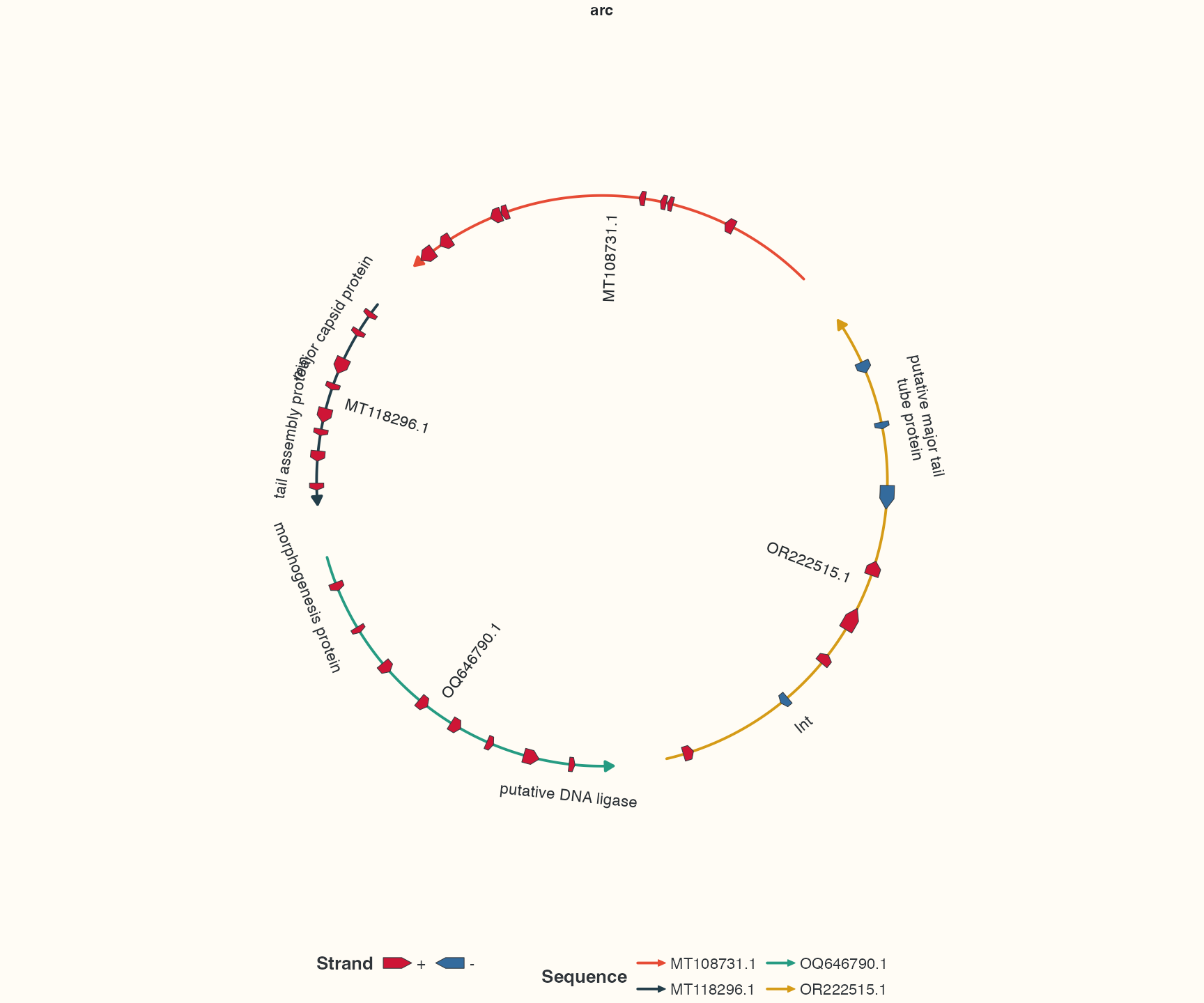
Data, code and interpretation →
p_labelarc · 12 × 10 in · 144 dpi
Explicit sequence, strand and query-category colour scales
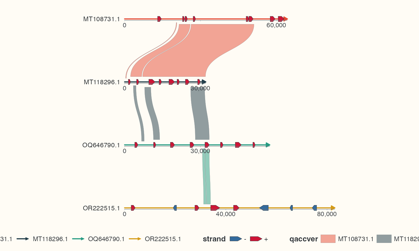
Data, code and interpretation →
p_styled · 10 × 6 in · 144 dpi
A real minimap2 PAF comparison between two EMALE genomes
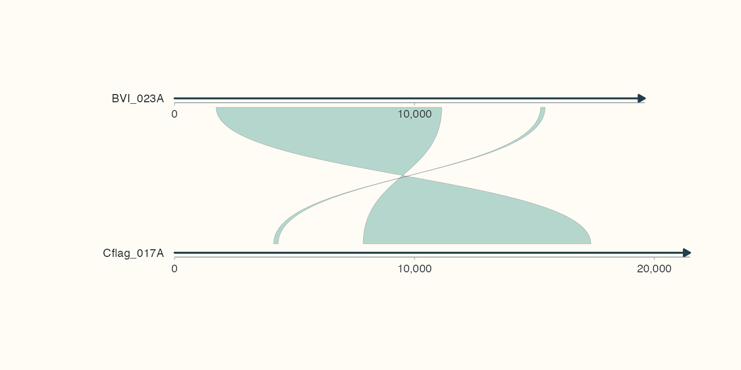
Data, code and interpretation →
p_paf · 10 × 5 in · 144 dpi
Your first plot: two bundled sequences, gene arrows and observed alignment intervals
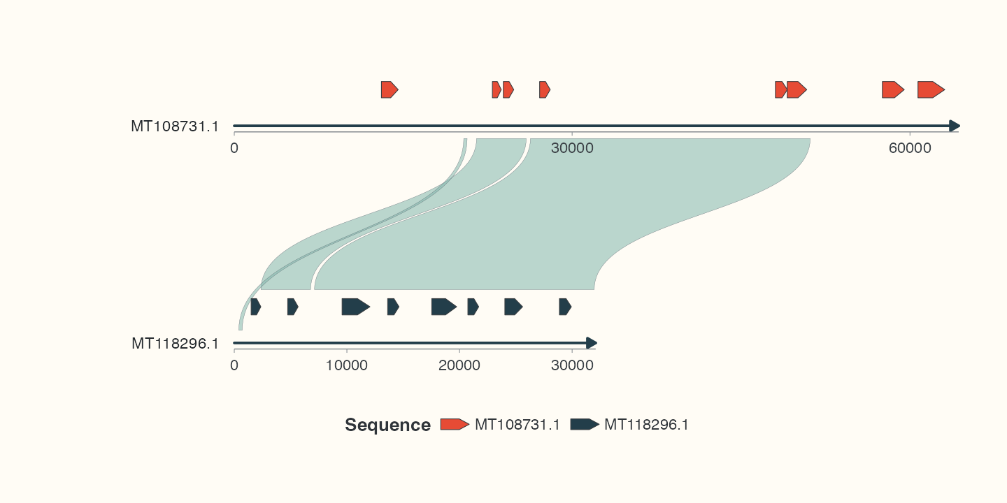
Data, code and interpretation →
p_first · 10 × 5 in · 144 dpi
Four-genome chord comparison with mixed backbone curvature and measured identity
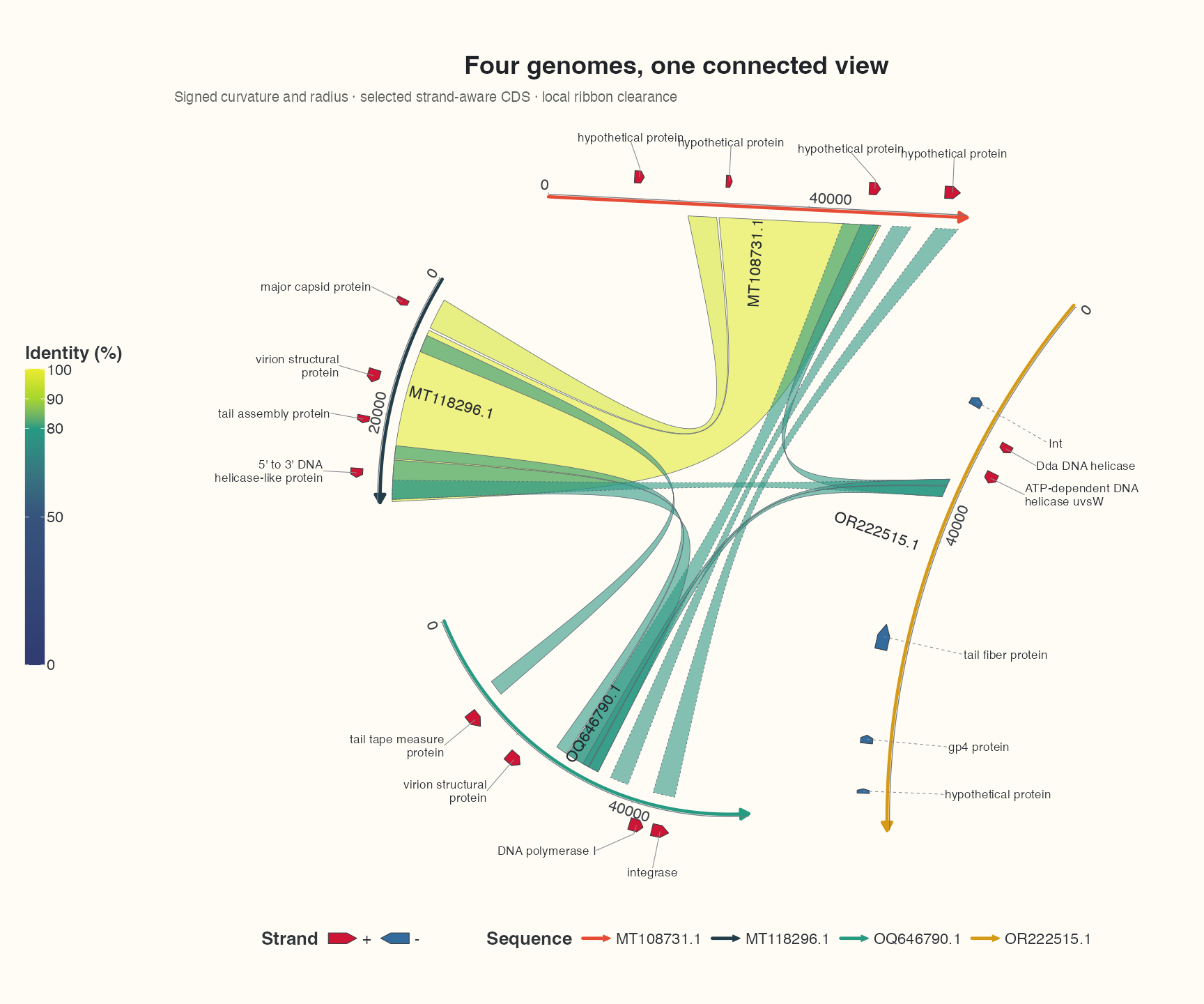
Data, code and interpretation →
p_show_chord · 12 × 10 in · 144 dpi
Dense pETDuet-1 map: features, reference primers and grouped restriction sites
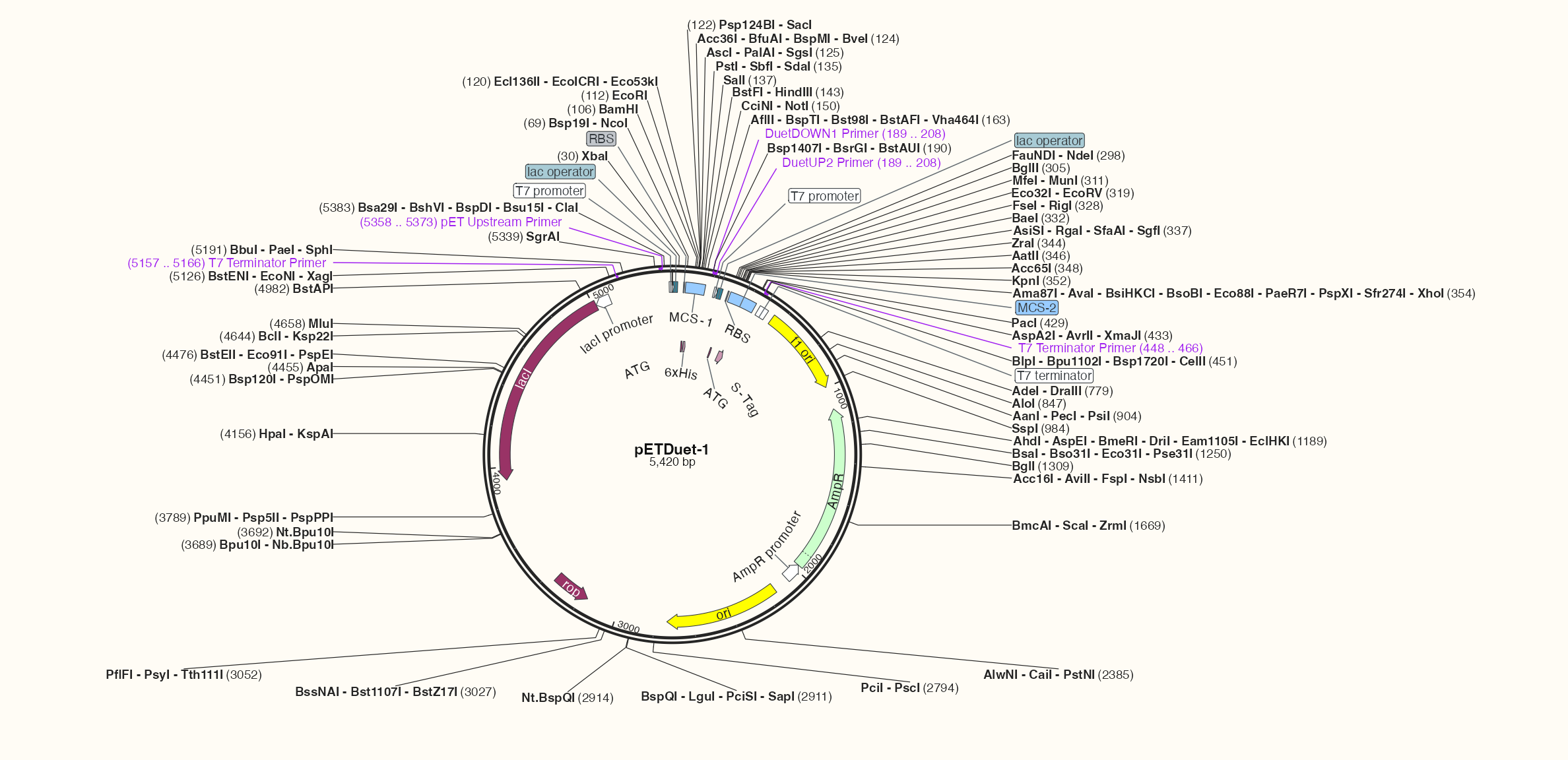
Data, code and interpretation →
p_show_plasmid · 16.5 × 8 in · 144 dpi
Four-genome collinearity: strand-separated features and routed cross-row links
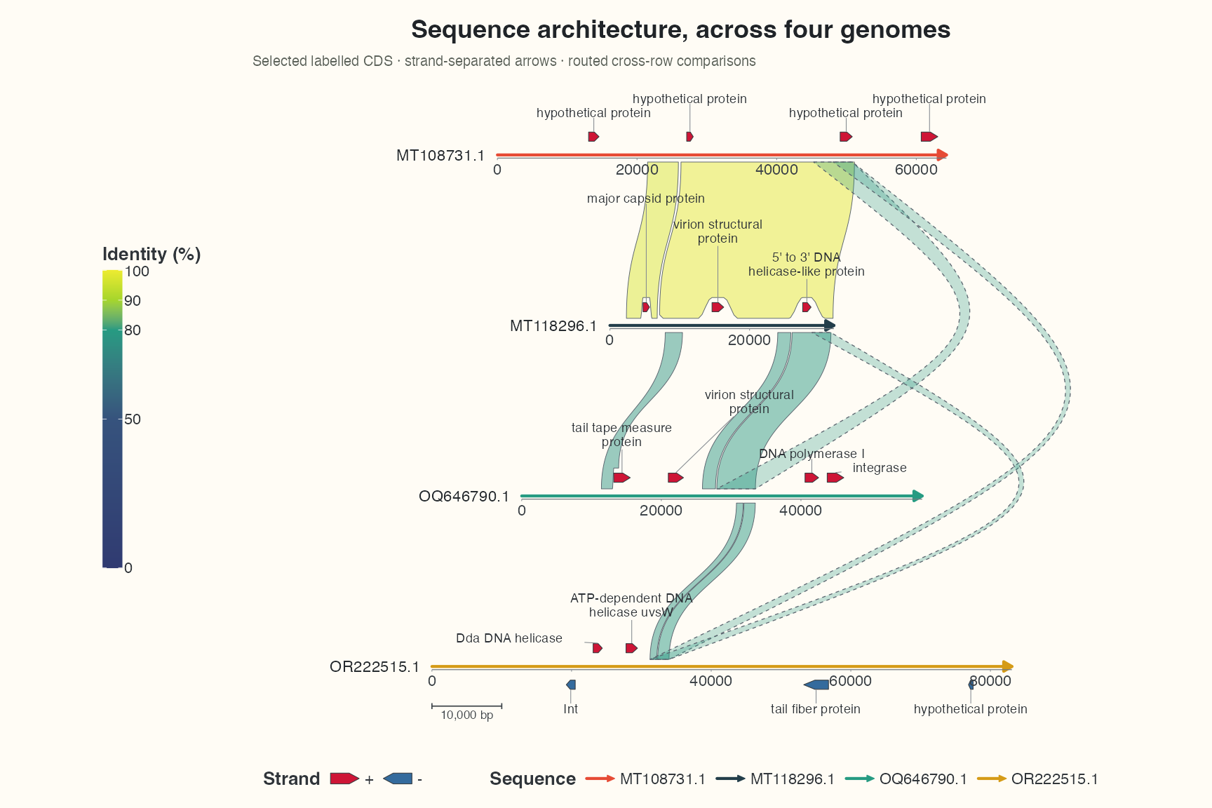
Data, code and interpretation →
p_show_collinear · 12 × 8 in · 144 dpi
Chord step1: sequence backbones
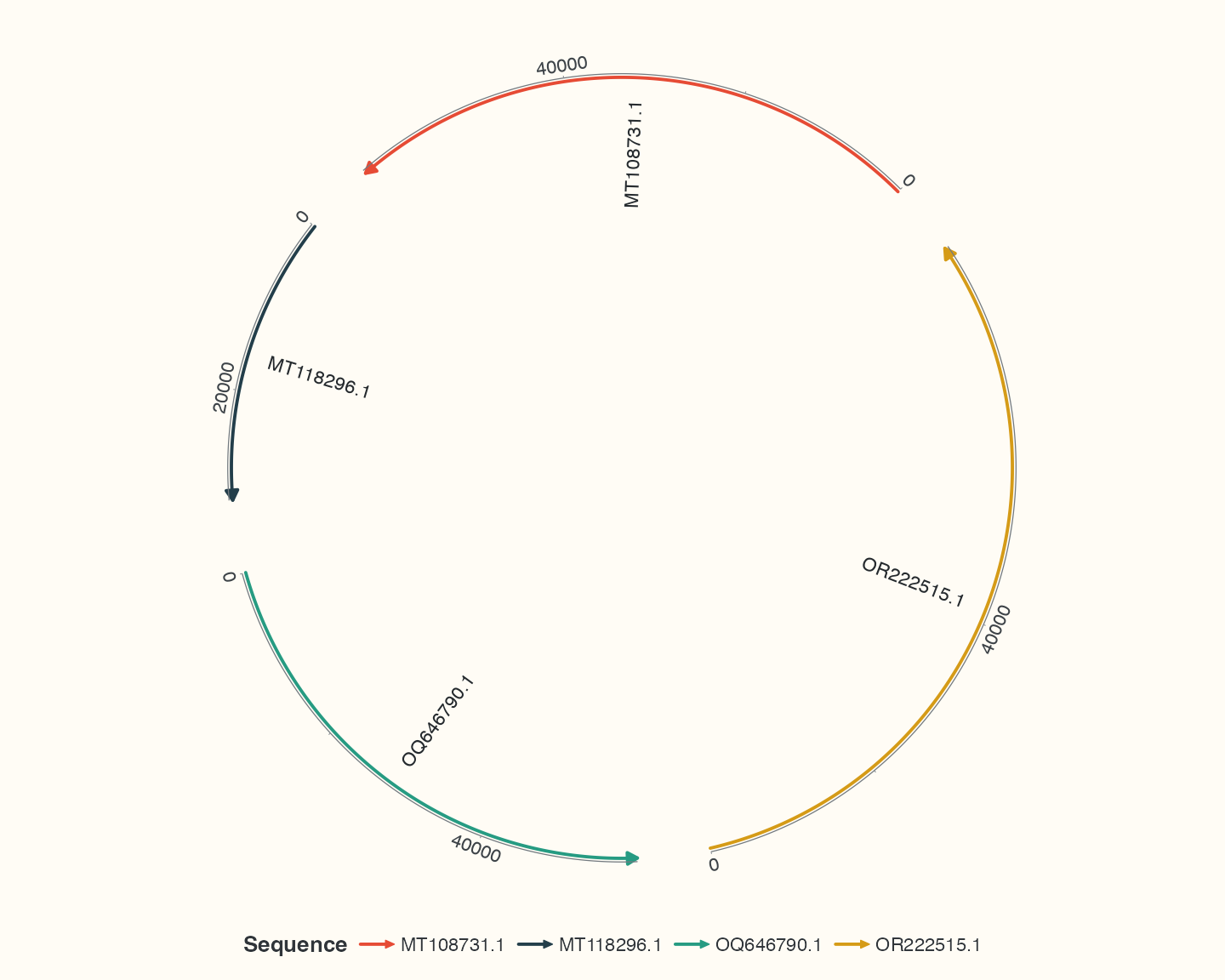
Data, code and interpretation →
p_learn_seq · 10 × 8 in · 144 dpi
Chord step2: observed comparisons
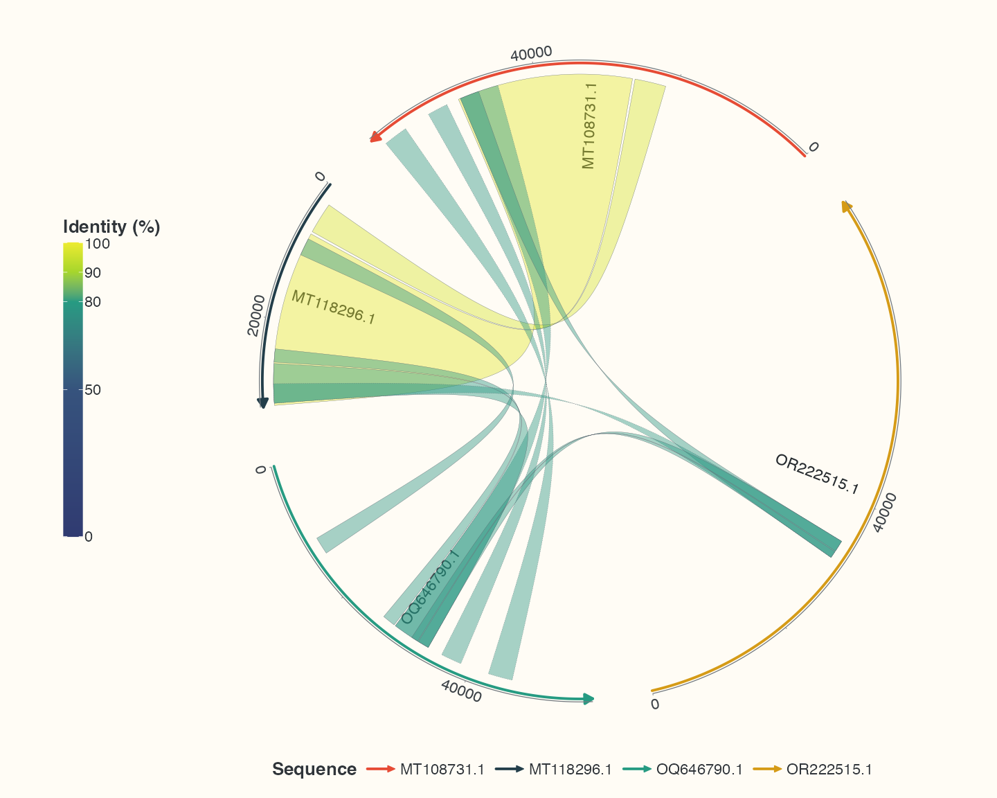
Data, code and interpretation →
p_learn_links · 10 × 8 in · 144 dpi
Chord step3: selected genes
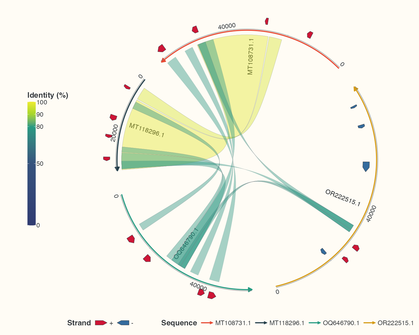
Data, code and interpretation →
p_learn_genes · 10 × 8 in · 144 dpi
Chord step4: labels for selected features
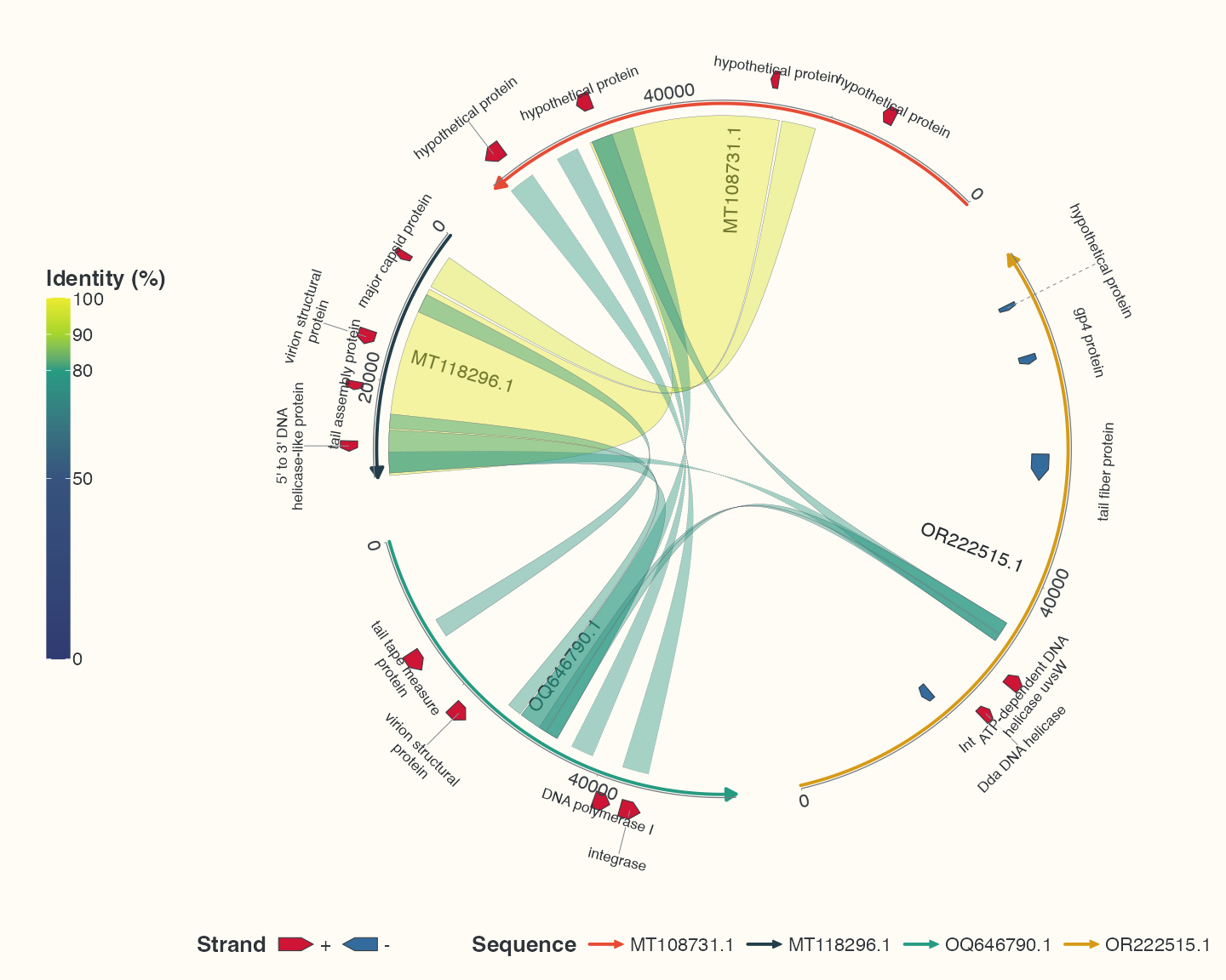
Data, code and interpretation →
p_learn_labels · 10 × 8 in · 144 dpi
The same backbones with linear coordinates
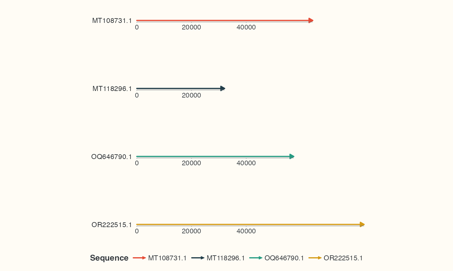
Data, code and interpretation →
p_linear_seq · 10 × 6 in · 144 dpi
The same observed links with linear coordinates
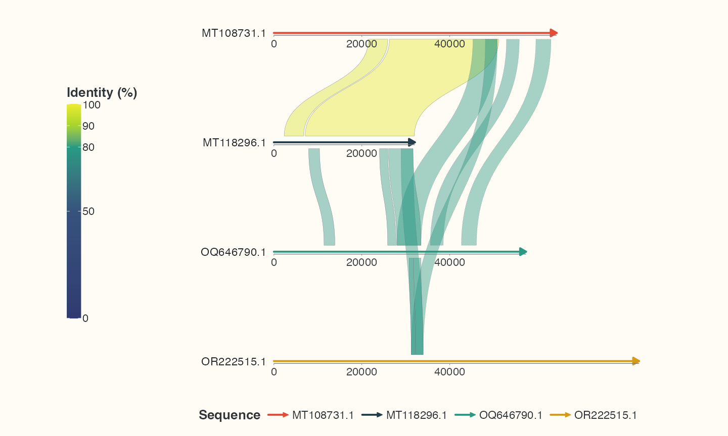
Data, code and interpretation →
p_linear_links · 10 × 6 in · 144 dpi
The same genes and labels with linear coordinates
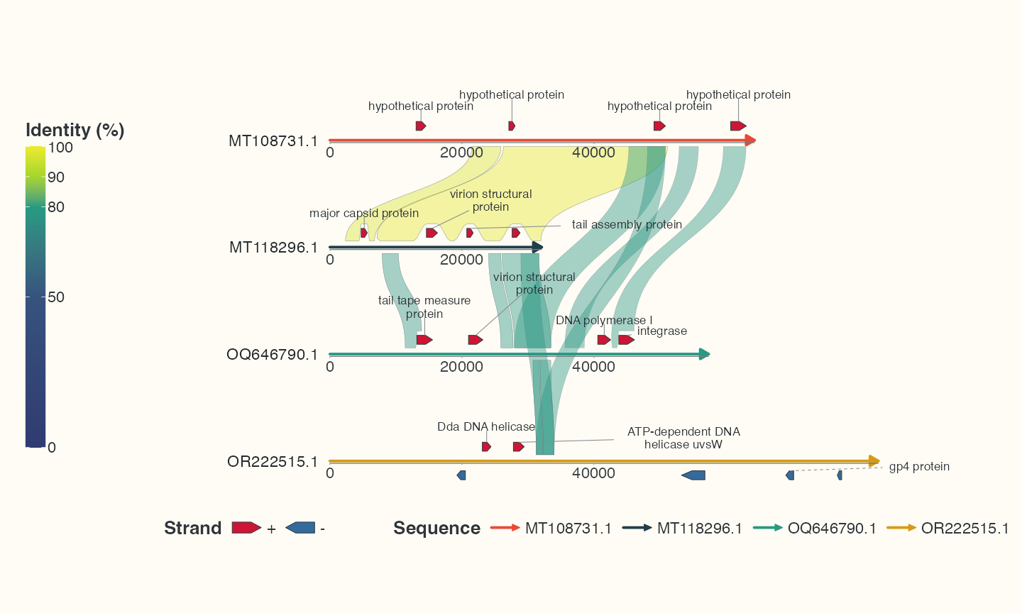
Data, code and interpretation →
p_linear_labels · 10 × 6 in · 144 dpi
pUC19 step1: double backbone
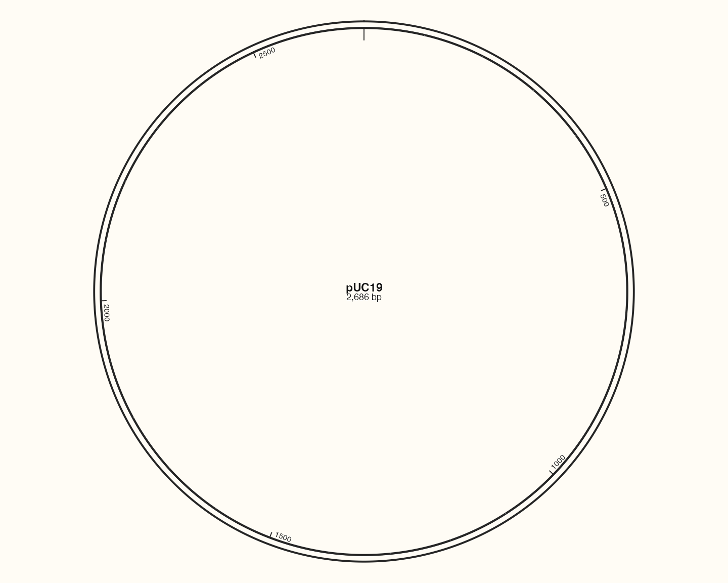
Data, code and interpretation →
p_plasmid_backbone · 10 × 8 in · 144 dpi
pUC19 step2: features
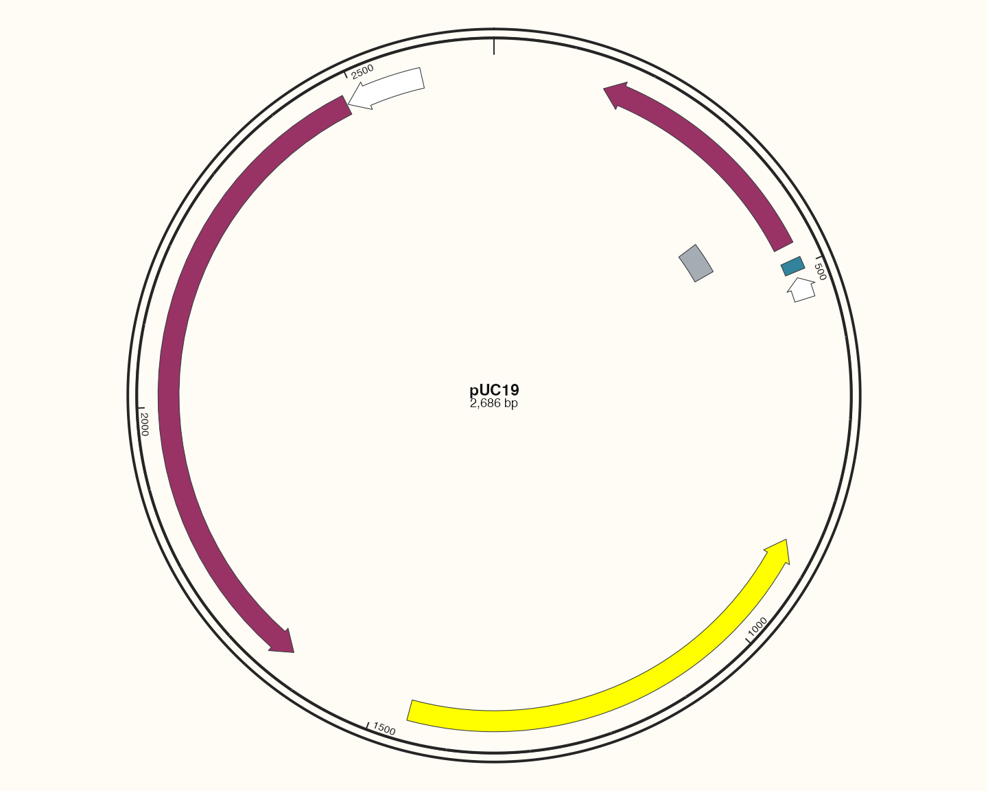
Data, code and interpretation →
p_plasmid_features · 10 × 8 in · 144 dpi
pUC19 step3: labels
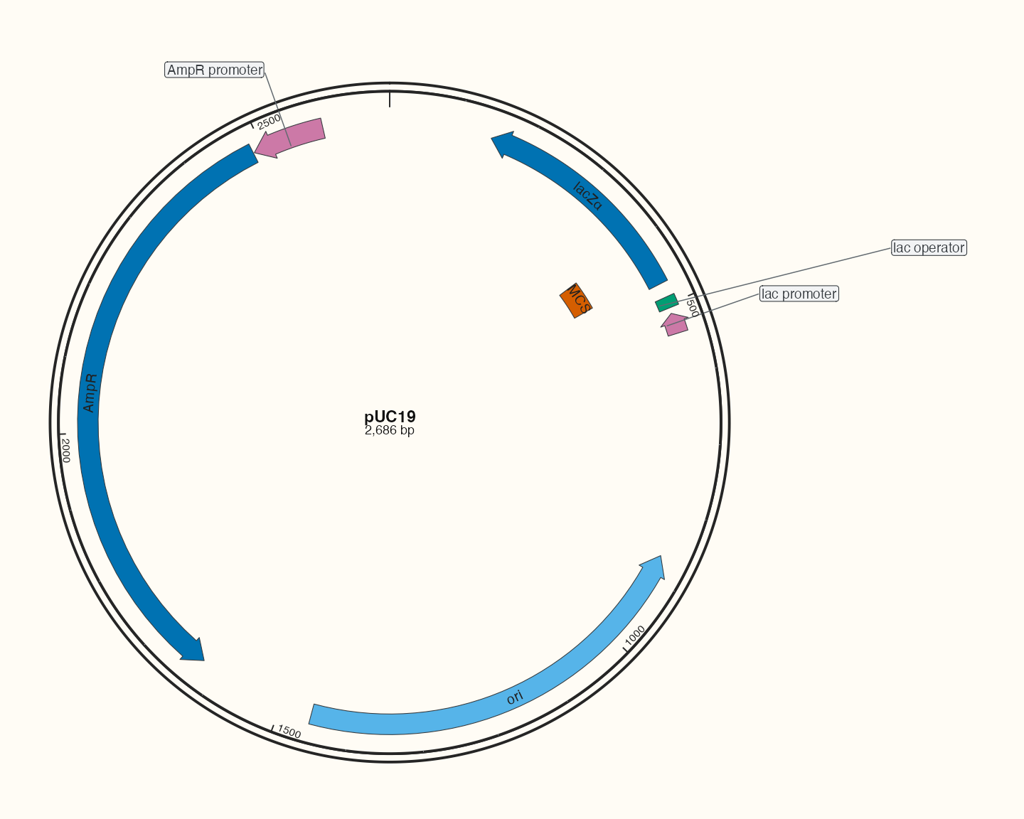
Data, code and interpretation →
p_plasmid_text · 10 × 8 in · 144 dpi
pSB1C3: source-backed feature map
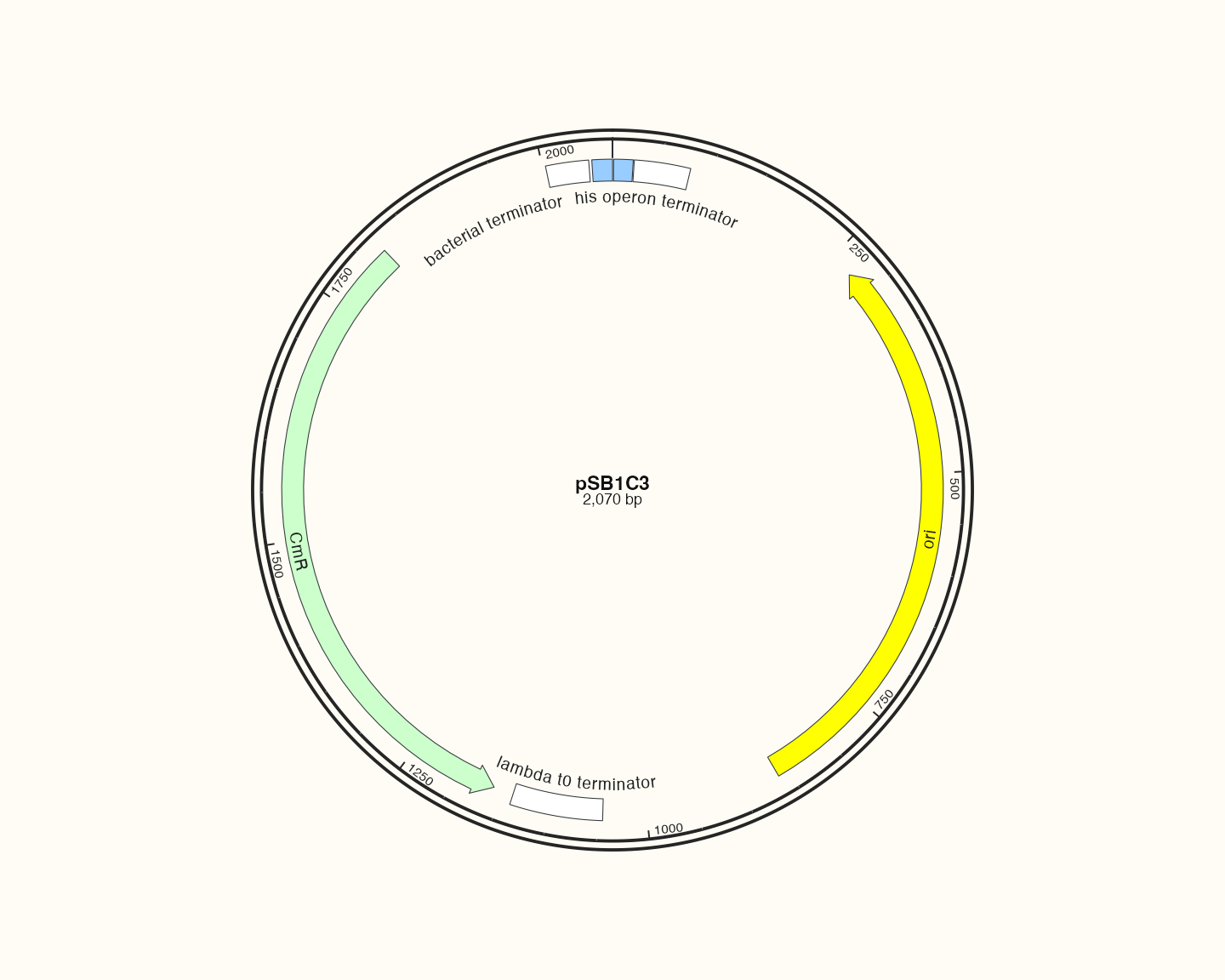
Data, code and interpretation →
p_catalogpsb · 10 × 8 in · 144 dpi
pUC19: source-backed feature map
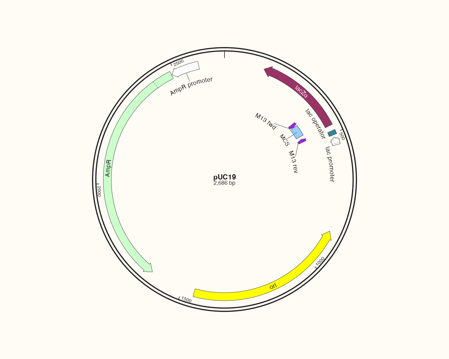
Data, code and interpretation →
p_catalogpuc · 10 × 8 in · 144 dpi
pBR322: source-backed feature map
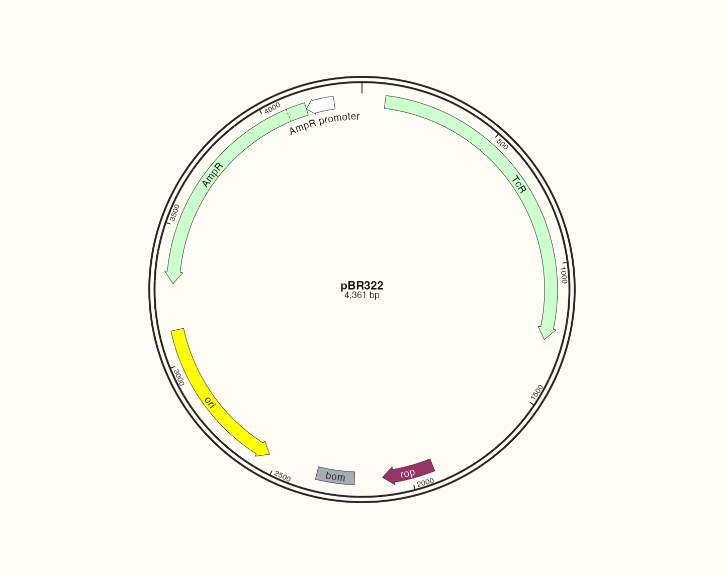
Data, code and interpretation →
p_catalogpbr · 10 × 8 in · 144 dpi
pBluescript II SK(+): source-backed feature map
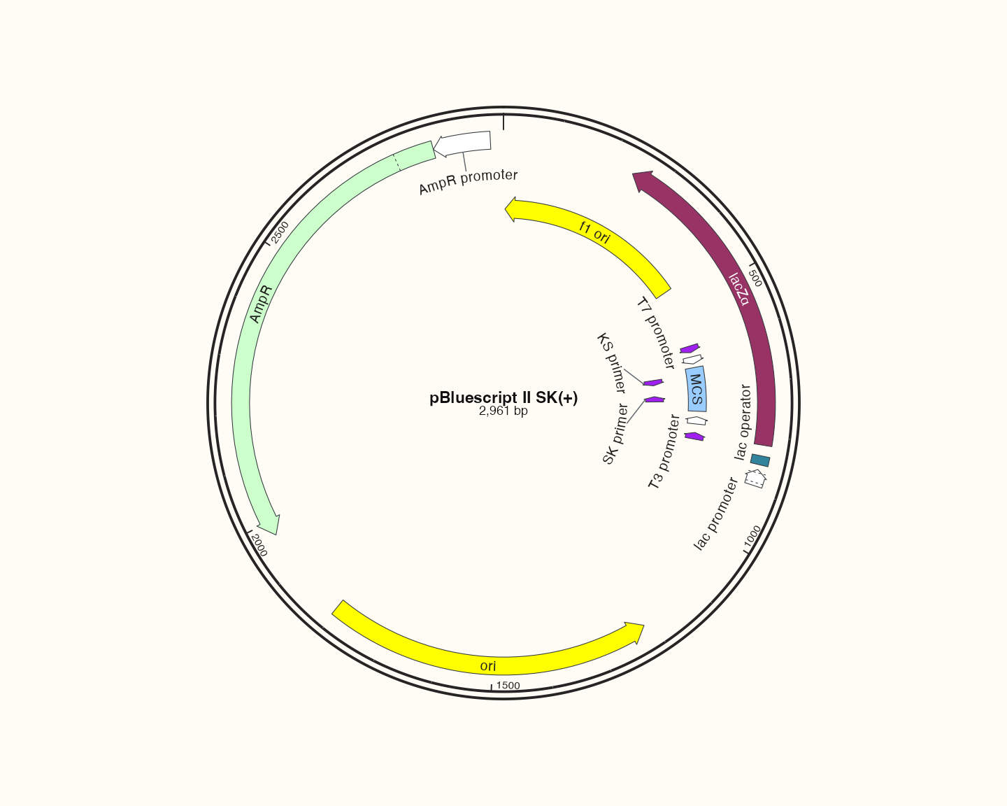
Data, code and interpretation →
p_catalogblue · 10 × 8 in · 144 dpi
pET-28a(+): source-backed feature map
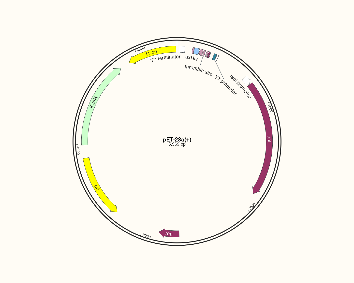
Data, code and interpretation →
p_catalogpet · 10 × 8 in · 144 dpi
pETDuet-1: source-backed feature map
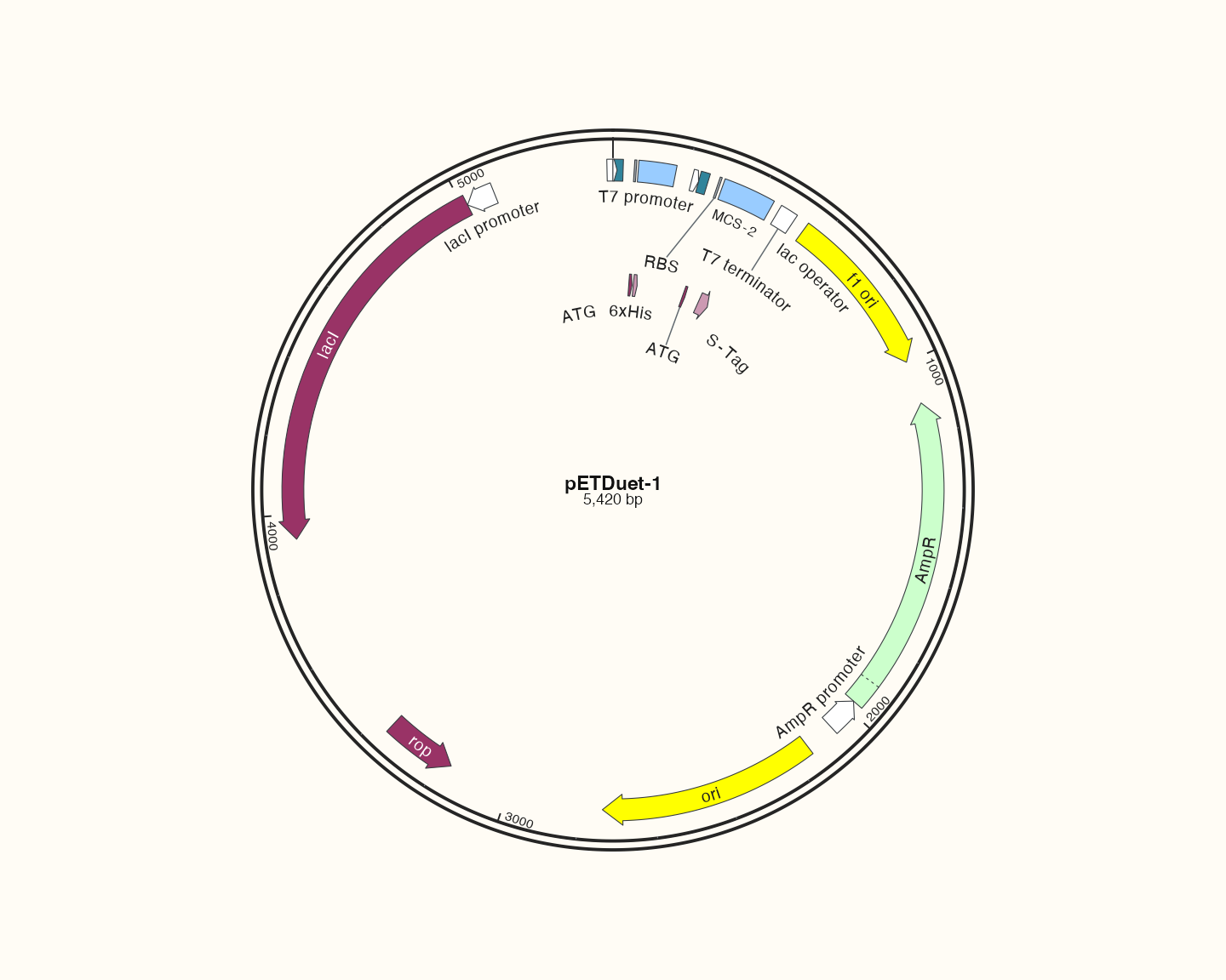
Data, code and interpretation →
p_catalogduet · 10 × 8 in · 144 dpi
pDONR221: source-backed feature map
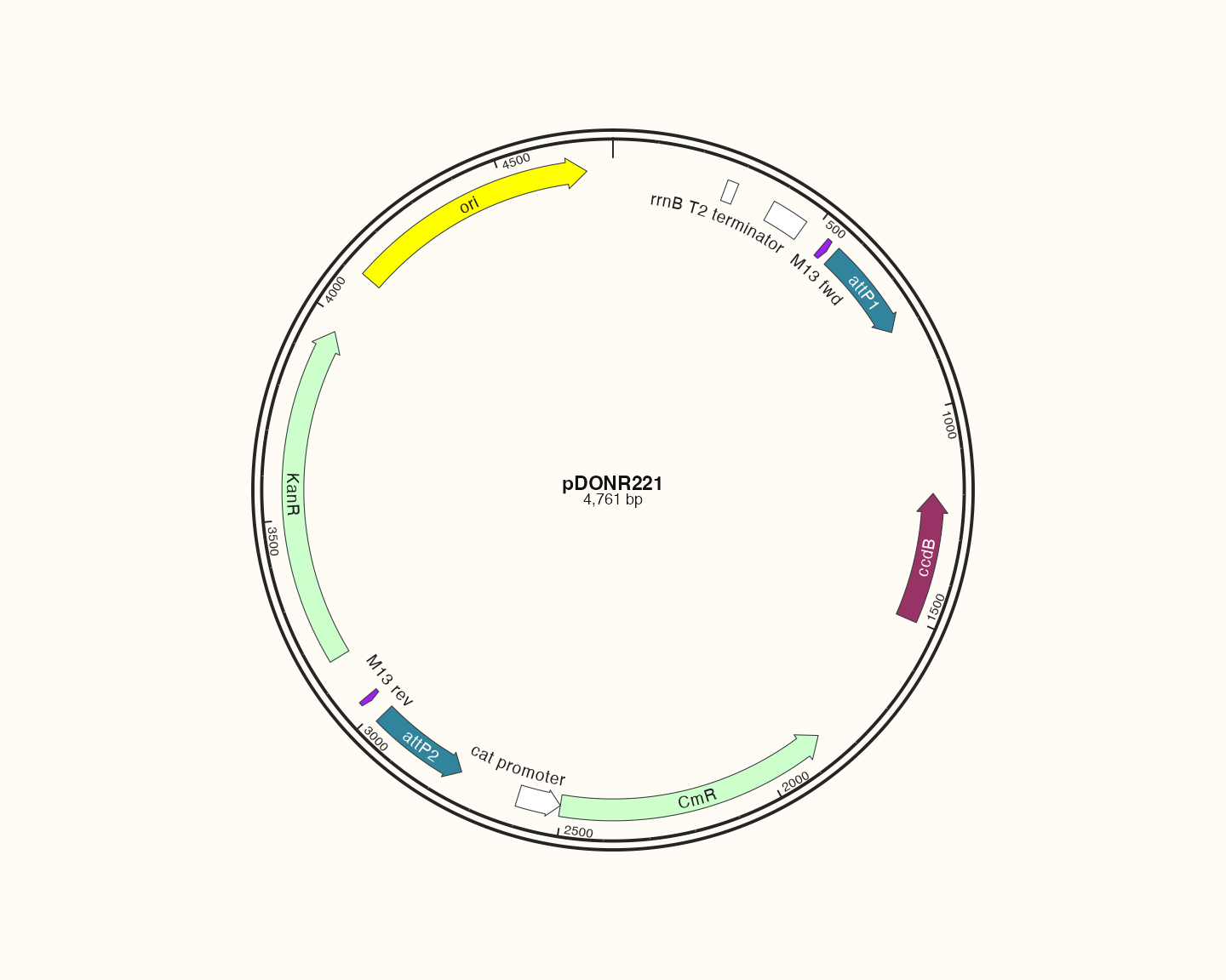
Data, code and interpretation →
p_catalogdonr · 10 × 8 in · 144 dpi
pcDNA3.1(+): source-backed feature map
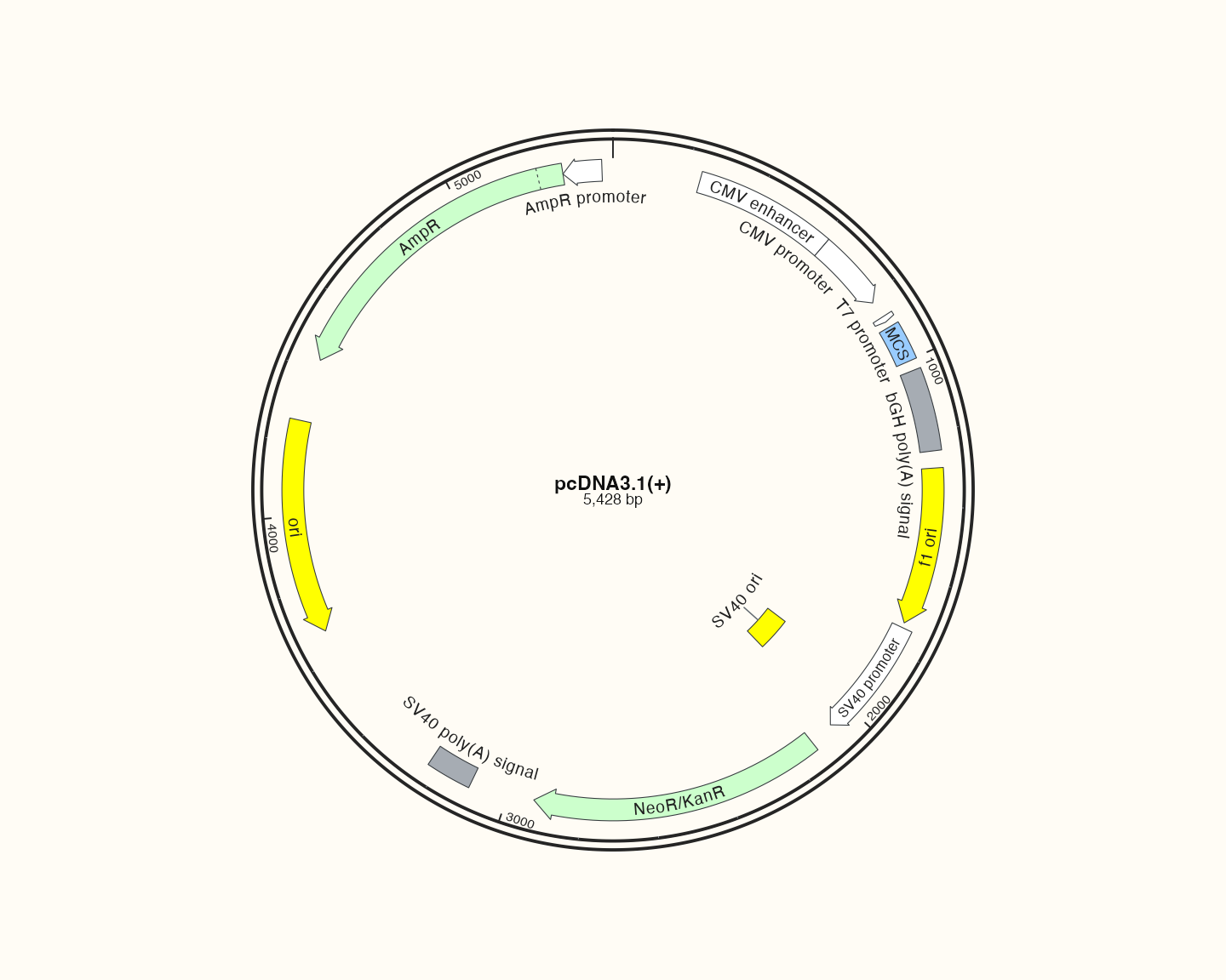
Data, code and interpretation →
p_catalogpcdna · 10 × 8 in · 144 dpi
pTRE-Tight-BI: source-backed feature map
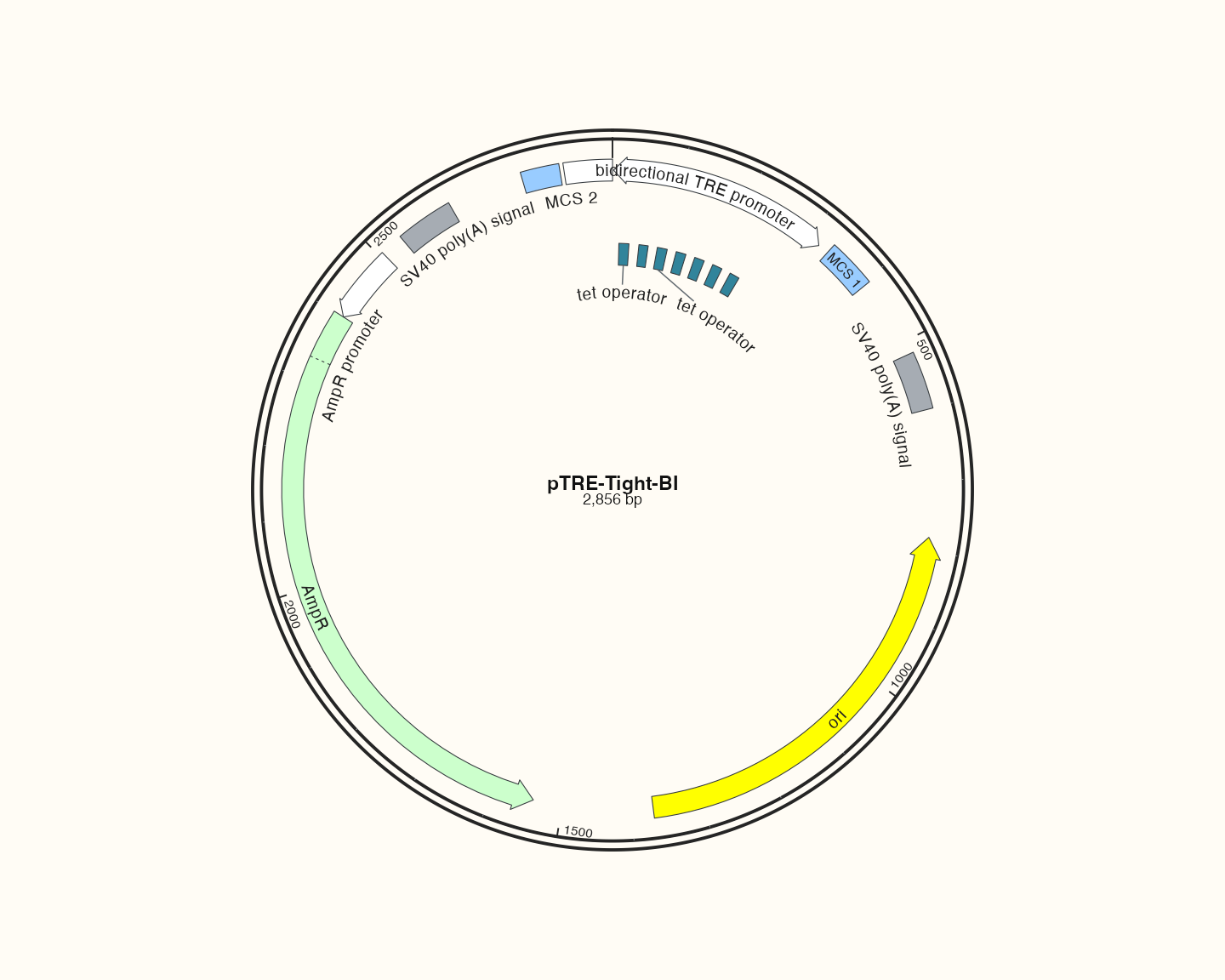
Data, code and interpretation →
p_catalogtre · 10 × 8 in · 144 dpi
pTRIPZ: source-backed feature map
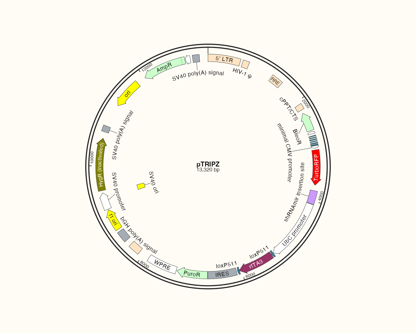
Data, code and interpretation →
p_catalogtripz · 10 × 8 in · 144 dpi
pCAMBIA1300: source-backed feature map
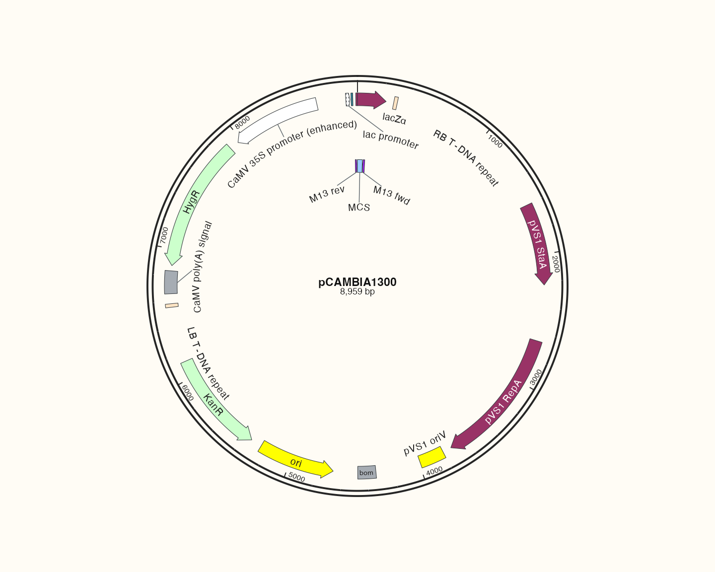
Data, code and interpretation →
p_catalogcambia · 10 × 8 in · 144 dpi
pEarleyGate 201: source-backed feature map
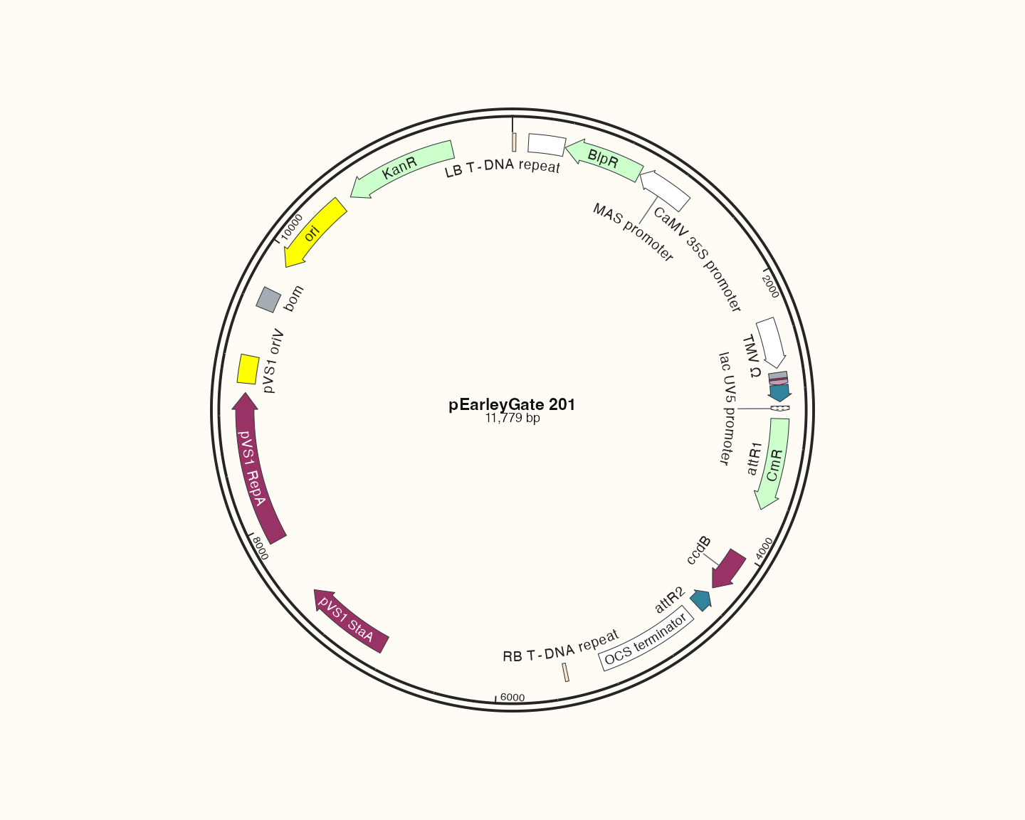
Data, code and interpretation →
p_catalogearley · 10 × 8 in · 144 dpi
pSpCas9(BB)-2A-GFP (PX458): source-backed feature map
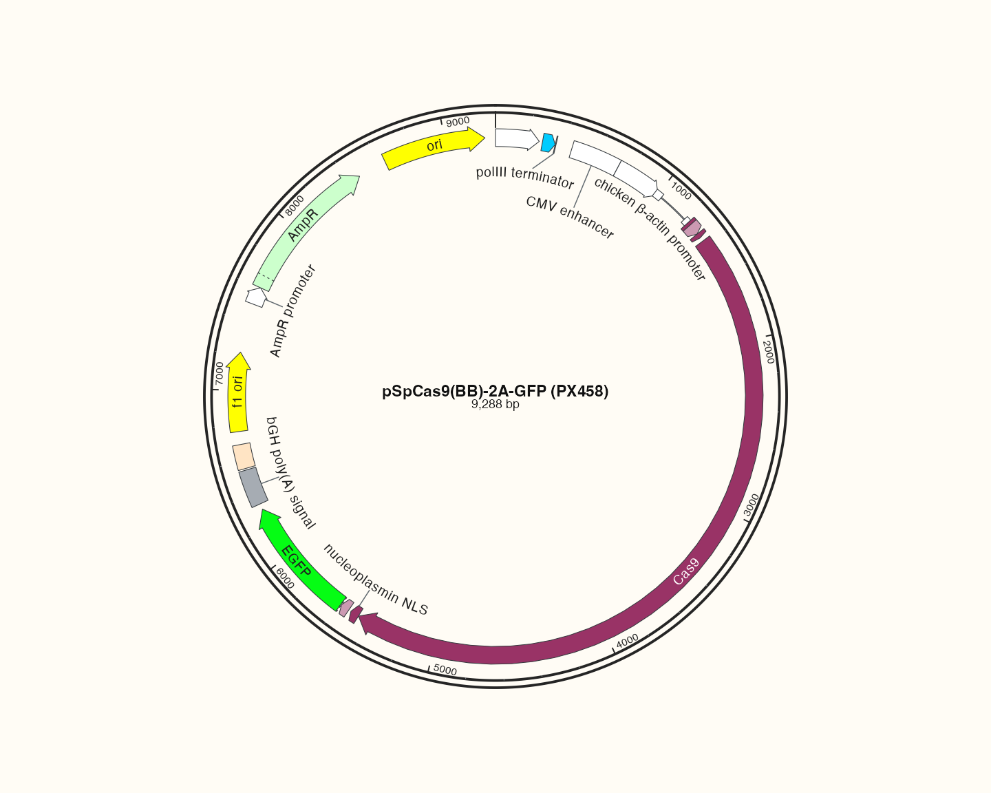
Data, code and interpretation →
p_catalogcas · 10 × 8 in · 144 dpi
One source for both languages
All figures use bundled source-backed data or attributed real input records, defined in the shared documentation example source. No raw FASTA/GFF3/BLAST record was changed to improve appearance. The same image bytes are used by both languages, README and vignette; captions provide localized interpretation. The source and asset hashes are recorded in the asset manifest.
Display filters are stated in the relevant articles. GC is computed from actual DNA; exact-CDS membership is checked from sequence content. Deliberate corruption is confined to diagnostic examples and is never presented as biological data.
Reproduce
From the source repository, with its suggested development dependencies available:
Code
Rscript tools/documentation-plots.R
python3 tools/sync-tutorials.py --check
python3 tools/build-website.py
python3 tools/check-documentation.py
The PNG device is used only to update these documentation figures. This is not an output-device matrix or release validation. Source code and dimensions live in tools/documentation-plots.R; changing the figure parameters requires regenerating the manifest. See output for your own export.