Chapters and reference
Module I · Multi-sequence relationships · Section 2 of 16
1.1 Shared data and layers
On this page
Build backbones, a link, a feature and labels in one section using bundled source records. Run in order; this section uses ggchord and optional dplyr.
1 Draw the backbones
Run this section in a fresh R session after following the installation instructions.
R · Example code
p_chord_backbone <- ggchord(seq_data = seq_data_example) +
  geom_seq() +
  geom_seq_label() +
  coord_chord()
view_ggchord(p_chord_backbone, width = 7, height = 7, units = "in")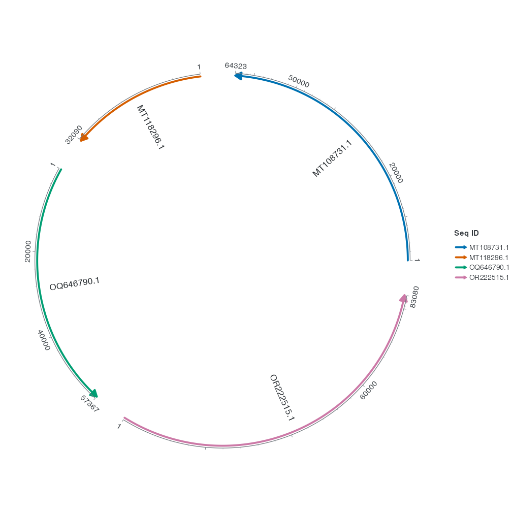
2 Read the plot
Each arc represents a row of the sequence table. Find MT108731.1 by its label and compare it with MT118296.1. These two sequences are 64,323 bp and 32,090 bp, so the first arc is about twice as long as the second.
geom_seq() draws the backbones, geom_seq_label() adds their IDs, and coord_chord() arranges the backbones as arcs.
3 What the label layer controls
Remove the geom_seq_label() line and run the code again. The arcs stay in place and the sequence names disappear.
4 Add an alignment ribbon
Take the first row of the bundled alignment table. It connects two of the four sequences.
R · Example code
chord_links <- head(ribbon_data_example, 1)

p_chord_ribbon <- p_chord_backbone +
  geom_link_ribbon(data = chord_links)
view_ggchord(p_chord_ribbon, width = 7, height = 7, units = "in")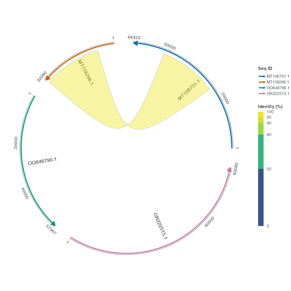
Follow the ribbon to both ends. It spans 26,298–51,139 bp on MT108731.1 and 7,121–31,959 bp on MT118296.1. Each end covers an interval, so this layer uses geom_link_ribbon().
The default colour reflects the alignment identity for this row, about 98.6%. The crossed shape comes from how the interval ends are joined. Use the alignment coordinates to assess inversion.
5 Add a CDS
Select the original annotation starting at 43,765 bp on OQ646790.1 and recover its biological strand.
R · Example code
chord_genes_example <- subset(gene_data_example, accver == "OQ646790.1" & start == 43765)
chord_genes_example$strand <- chord_genes_example$source_strand

p_chord_feature <- p_chord_ribbon +
  geom_gene(data = chord_genes_example)
view_ggchord(p_chord_feature, width = 7, height = 7, units = "in")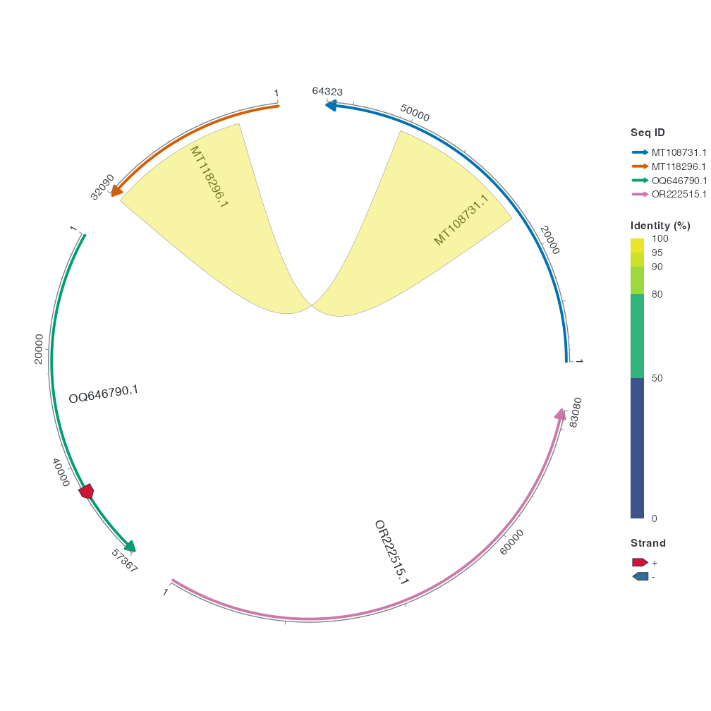
Find the red arrow on green OQ646790.1. It marks the plus-strand integrase CDS from 43,765 to 46,140 bp. The ribbon and this CDS use independent input tables.
To display the CDS name, add geom_gene_label(data = chord_genes_example). It reads the label from anno.
6 Display the feature name
R · Example code
p_chord_gene_labels <- p_chord_feature +
  geom_gene_label(data = chord_genes_example, label_radial_offset = 0.10)
view_ggchord(p_chord_gene_labels, width = 7, height = 7, units = "in")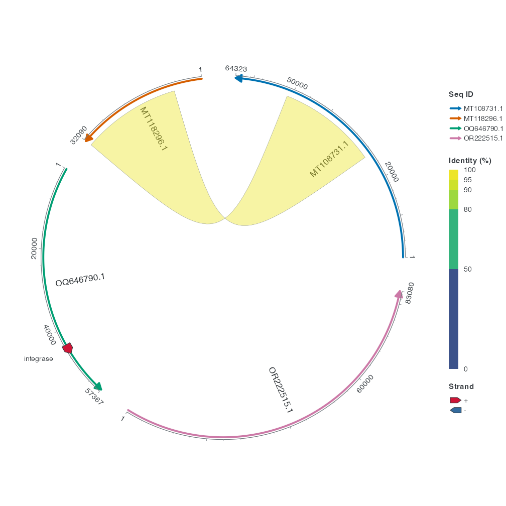
7 Switch to a linear layout
R · Example code
p_chord_linear <- p_chord_gene_labels + coord_collinear()
view_ggchord(p_chord_linear, width = 8, height = 5, units = "in")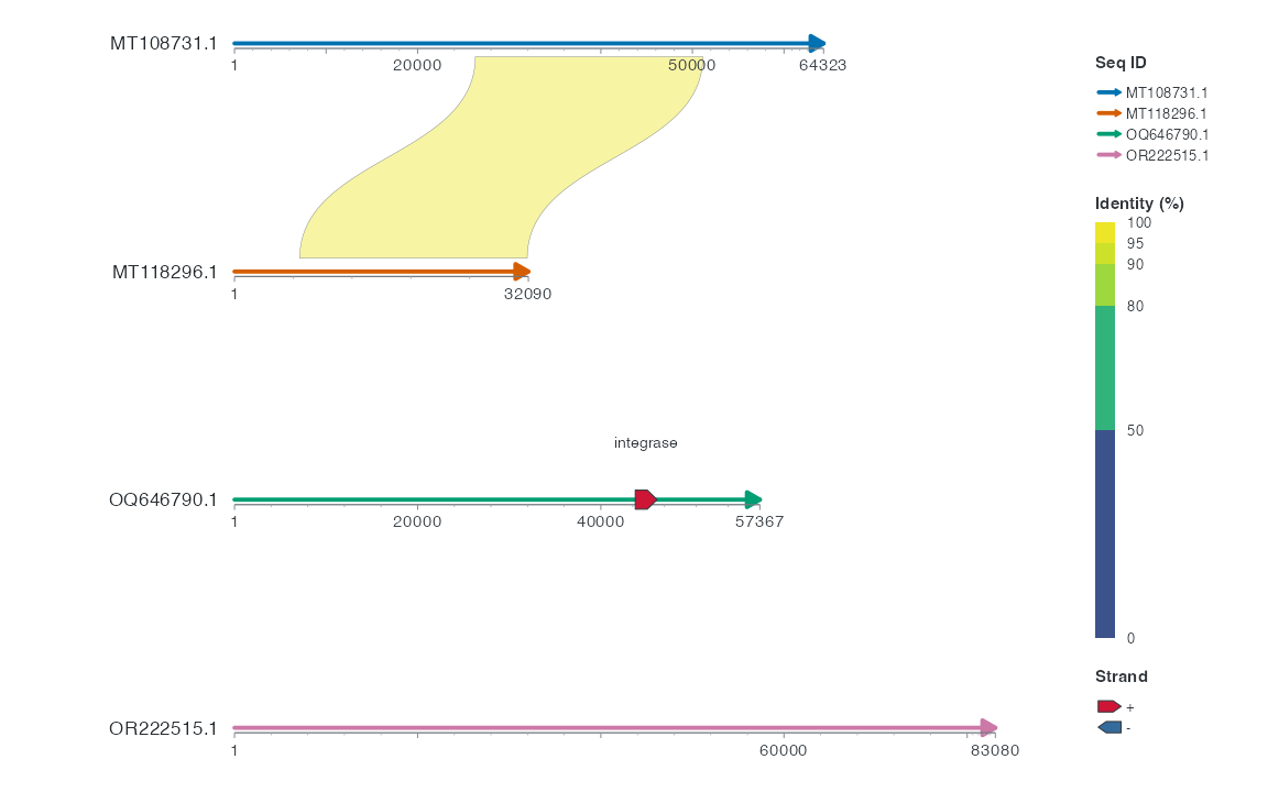
This retains the ribbon, CDS and feature-name layers; Collinear selects adjacent rows by default. Compare all four views in the next section.
8 Use your own sequences
Replace seq_data_example with a table containing accver and length. See Basic input tables for the column definitions, Flexible parameter formats for local settings, and Four-view comparison for a strict coordinate comparison.