0.16.6 documentation

Site guide · find your task

Setup and learning paths

HomeInstall and prepare the environmentChoose your learning module

Module I · Chord

1.1 Tables and field meanings1.2 Produce and import comparisons1.3 Build the layers step by step1.4 Direction, curvature and clearance1.5 Filter and summarize links1.6 Full source-file workflow1.7 Complete chord showcase

Module II · Collinear

2.1 Reuse chord input tables2.2 Switch coordinates and add layers2.3 Routes, clearance and the ruler2.4 Compare CDS neighbourhoods2.5 Focus, anchors and segments2.6 Complete collinear showcase

Module III · Plasmid

3.1 DNA, annotations and 13 references3.2 From a circle to annotation layers3.3 Features, primers and restriction3.4 Thirteen plasmid references3.5 Complete plasmid cases

Consult as needed · Data and layers

Prepare tables and coordinatesImport and convert dataImport nucleotide and protein alignmentsProject protein intervals to genomic coordinatesFeatures, stacking and genomic decorationLabels and local placementQuantitative tracksMappings, scales, guides and themesSet values by sequence and strandCommon adjustments and grammarExport, preview and diagnostics

Learning map and reference

Articles and complete workflowsFunction referenceReproducible galleryFrequently asked questionsMigrate to the candidate APITerminology and design sourcesDevelopment status and changes

1.6 Full source-file workflow

On this page

• Prepare this page
• 1. Read and inspect original records
• 2. Make the display selection explicit
• 3. Build a chord comparison
• 4. Inspect all annotations in a linear view
• 5. Keep the evidence with the figure
• Select fields before passing data
• Check your result
• Save this result

Combine original FASTA, GFF3 and standard BLAST tables into a traceable comparison. Inspect inputs, choose a display subset, then compare chord and full-length views.

Prepare this page

In a fresh R session, run the code below, then follow this page in order. Colours and layout are optional display choices; inputs select only the fields needed. For file-based examples, first extract the input bundle so the working directory contains examples/.

Preparation code — run once on this page

Code

# Optional appearance choices; none of these columns or scales is required input.
library(ggchord)
seq_palette <- setNames(
  c("#E64B35", "#233E4A", "#269B82", "#D59B17"),
  c("MT108731.1", "MT118296.1", "OQ646790.1", "OR222515.1")
)
gene_palette <- c("+" = "#CE1536", "-" = "#346B9D", "." = "#8291A6")

library(ggchord)
doc_background <- "#FFFCF5"
identity_palette <- c("#303B71", "#36537D", "#269B82", "#A5D52C", "#ECEB31")
identity_values <- c(0, 0.5, 0.8, 0.9, 1)
identity_breaks <- c(0, 50, 80, 90, 100)
doc_legend_theme <- theme(
  legend.title = element_text(size = 13, face = "bold"),
  legend.text = element_text(size = 11),
  legend.key.width = unit(9, "mm"), legend.key.height = unit(5, "mm"),
  legend.spacing.x = unit(9, "mm"), legend.spacing.y = unit(7, "mm"),
  legend.margin = margin(l = 4, r = 4, unit = "mm")
)
sequence_guide <- guide_ggchord_legend(nrow = 1, theme = doc_legend_theme)
strand_guide <- guide_ggchord_legend(
  nrow = 1, override.aes = list(strand = c("+", "-")), theme = doc_legend_theme
)
identity_guide <- guide_ggchord_colourbar(
  position = "left", direction = "vertical",
  theme = theme(
    legend.key.height = unit(75, "mm"), legend.key.width = unit(5, "mm"),
    legend.title = element_text(size = 13, face = "bold"),
    legend.text = element_text(size = 11), legend.margin = margin(r = 7, unit = "mm")
  )
)
doc_theme <- theme_ggchord_publication(
  axis.text = element_text(size = 11),
  axis.text.check.overlap = TRUE
) +
  theme(
    legend.position = "bottom",
    legend.title = element_text(size = 13, face = "bold"),
    legend.text = element_text(size = 11),
    legend.key.width = unit(9, "mm"), legend.key.height = unit(5, "mm"),
    legend.spacing.x = unit(9, "mm"), legend.spacing.y = unit(7, "mm"),
    legend.box.spacing = unit(6, "mm"),
    plot.background = element_rect(fill = doc_background, colour = NA),
    panel.background = element_blank(),
    plot.title = element_text(face = "bold", size = 18),
    plot.subtitle = element_text(size = 10, colour = "#5C625A"),
    plot.margin = margin(14, 18, 14, 18)
  )
doc_axis <- function(coordinates = "relative") {
  scale_seq_position_continuous(
    coordinates = coordinates, n.breaks = 3, minor_breaks = NULL,
    labels = function(x) format(x, scientific = FALSE, big.mark = ",", trim = TRUE)
  )
}

This complete workflow uses four sequence records already present in the source repository. It requires the matching development checkout or the tutorial input bundle, not new alignments or external gene prediction. Download the inputs and unpack them so examples/ is under the working directory. Record the package version and build manifest with the exported figure.

1. Read and inspect original records

Code

library(dplyr)
sequence_source <- read_fasta_lengths(files = "examples/fasta/*.fna", source_file = TRUE)
seq_real <- sequence_source |>
  select(accver, length)
annotation_source <- read_gff3(files = "examples/gff3/*.gff3", unstranded = "keep", source_file = TRUE)
feature_real <- annotation_source |>
  select(accver, start, end, strand, type, anno)
alignment_source <- read_blast(files = "examples/blastn-standard/*.tsv", source_file = TRUE)
link_real <- alignment_source |>
  select(qaccver, saccver, qstart, qend, sstart, send, pident, length)
real_validation <- validate_ggchord_data(seq_real, link_real)
real_validation

The FASTA headers supply exact accession versions and lengths. GFF3 contributes CDS intervals and their original strands. BLAST output contributes existing alignments; the reader does not run BLAST. Inspect real_validation before continuing: decreasing link endpoints can be legitimate reverse-direction hits. Never turn unknown annotation strands into + to make a gene shortcut accept them.

2. Make the display selection explicit

Code

real_prepared <- prepare_ggchord_data(seq_real, link_real,
  features = list(annotation = feature_real)
)
real_filtered <- filter_ggchord_ribbons(link_real, min_pident = 80, min_length = 500)
# Explicit display subset: the six longest CDS per sequence; raw annotations stay intact.
real_display_features <- feature_real |>
  group_by(accver) |>
  slice_max(end - start + 1, n = 6, with_ties = FALSE) |>
  ungroup()
real_labels <- real_display_features |>
  filter(anno != "hypothetical protein") |>
  group_by(accver) |>
  slice_head(n = 2) |>
  ungroup()
real_filtered$report

Metric	Observed output
Sequences	4
Annotation rows	266
CDS selected for the chord view	24
Original HSPs	32
HSPs retained by the display filter	8
Selected text labels	6

The link display retains identity ≥80% and reported alignment length ≥500 bp. The chord view selects the six longest imported CDS per sequence, labelling at most two selected CDS with informative annotations (excluding hypothetical protein). These are display rules, not biological findings or a claim that omitted genes are absent. Raw feature_real and link_real remain intact; real_prepared$report and real_filtered$report retain preparation/filter evidence. No display strands are recoded. This differs from the small packaged teaching fixture whose documented generation includes display-strand recoding.

3. Build a chord comparison

Code

p_real_chord <- ggchord(seq_data = seq_real, ribbon_data = real_filtered$data, validate = "none") +
  geom_link_ribbon(aes(ribbon_fill = pident), alpha = .65) +
  geom_seq(show.legend = FALSE) +
  geom_feature(aes(feature_fill = strand),
    data = real_display_features,
    width = .045, position = position_strand(.08)
  ) +
  geom_feature_label_repel(
    data = real_labels, label_layout = "radial",
    label_wrap = 20, size = 4, position = position_strand(.08)
  ) +
  geom_seq_label(size = 4, seq_label_radius = .84, seq_label_hjust = .5) +
  coord_chord() +
  scale_seq_colour_manual(values = seq_palette) +
  scale_feature_fill_manual(values = gene_palette, breaks = c("+", "-")) +
  scale_ribbon_fill_gradientn(
    colours = identity_palette, values = identity_values,
    limits = c(0, 100), breaks = identity_breaks, name = "Identity (%)", guide = identity_guide
  ) +
  doc_theme
p_real_chord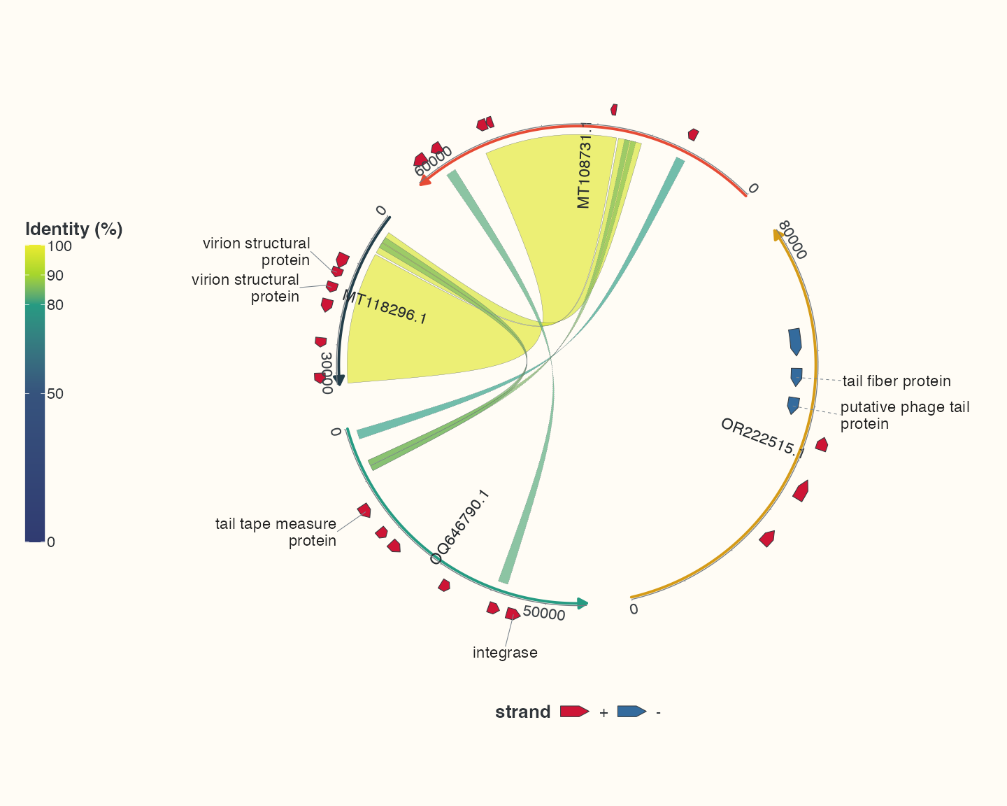

Original sequences with explicitly selected CDS and alignment links · Click to enlarge

Read sequence labels first, then source-strand feature arrows and interval links. Ribbons encode existing aligned intervals and mapped identity; their crossing is not itself evidence of a rearrangement. The selected features remain visibly separate from the much wider alignment spans. Use the full input tables when scientific interpretation needs annotations outside this display subset.

4. Inspect all annotations in a linear view

Code

p_real_linear <- ggchord(seq_real, real_filtered$data, validate = "none") +
  geom_link_ribbon(fill = "#6BAFA6", alpha = .45) +
  geom_seq() +
  geom_seq_label(size = 4) +
  geom_feature(data = feature_real, feature_fill = "#CE1536", show.legend = FALSE, position = position_strand(.18)) +
  geom_seq_scale(length = 10000) +
  coord_collinear() +
  doc_axis() +
  scale_seq_colour_manual(values = seq_palette) +
  doc_theme
p_real_linear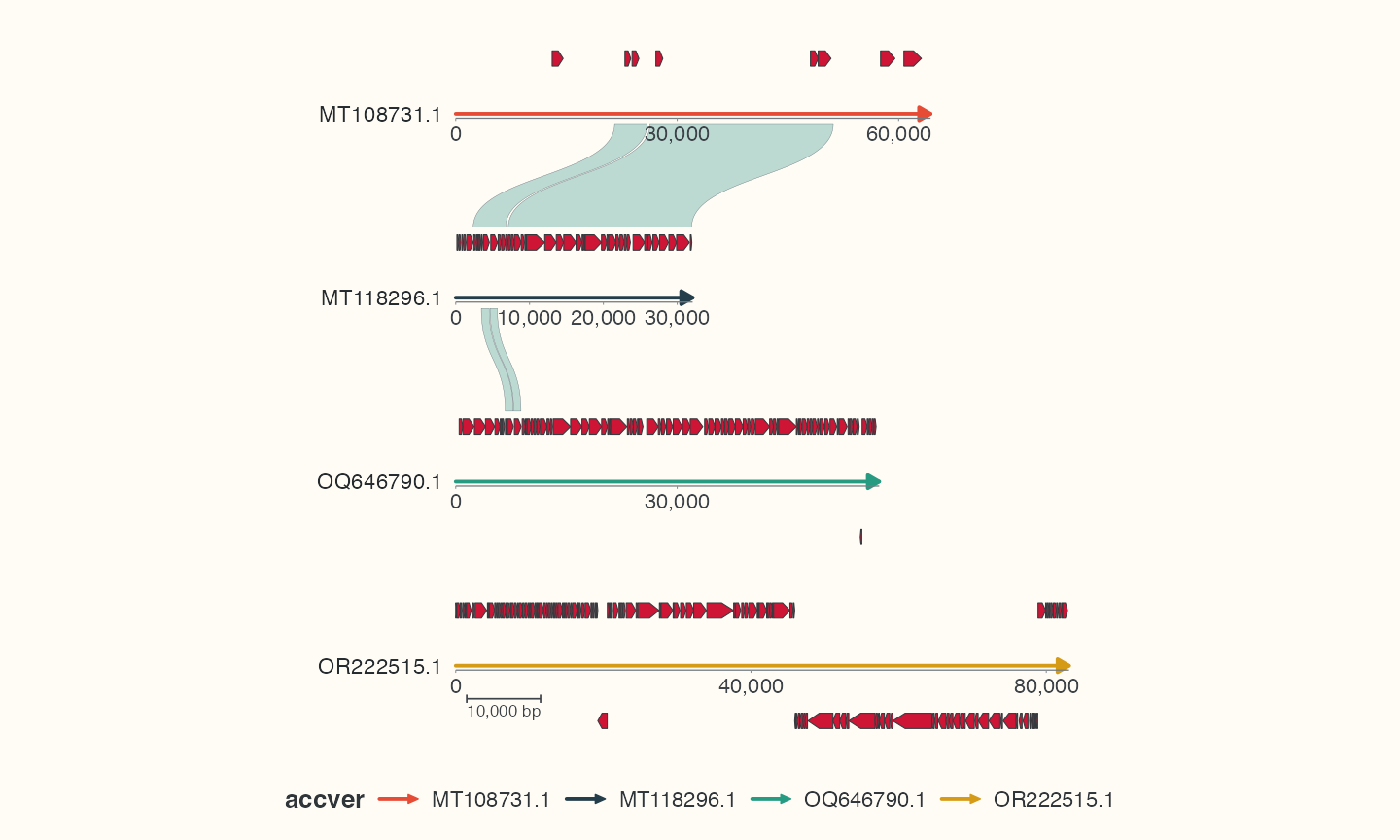

Original sequences, all imported CDS and filtered links · Click to enlarge

This view draws all imported annotations. Ribbons connect adjacent displayed sequences by default; retaining every comparison is an explicit layer decision. The bp scale bar belongs to collinear coordinates. See local views for cropping, source-coordinate axes and independent windows, and output to preview and save at the gallery’s stated dimensions.

5. Keep the evidence with the figure

The input archive contains unmodified FASTA/GFF3/BLAST files, a SHA256 manifest and the shared example script. The plot manifest records the code hash, PNG device, width, height and dpi. The accession names identify source records; a drawing is not a replacement for the original annotations or alignment evidence.

Select fields before passing data

The *_source objects keep original fields and provenance; seq_real has two columns, feature_real only geometry/type/text, and link_real adds identity and reported length only because this workflow filters and colours by them. Standard 12-column BLAST conversions are used, not a requirement for the historical 17 fields. The bundled gene fixture preserves its original strand in source_strand; the short examples restore that biological strand before selecting four gene columns. See alignment input for exact format and unit boundaries.

Check your result

Check that IDs agree across the tables, inspect filtering reports and verify that guides encode identity and strand. Use the overview to locate regions, then focus a neighbourhood to study a CDS.

Continue: Explicit homologs and coding-coordinate links →

Save this result

Save the plot just created to the working directory; use matching dimensions for preview.

Code

ggsave("phage-comparison.png", p_real_chord, width = 10, height = 8, units = "in", dpi = 144)