0.16.6 documentation

Site guide · find your task

Setup and learning paths

HomeInstall and prepare the environmentChoose your learning module

Module I · Chord

1.1 Tables and field meanings1.2 Produce and import comparisons1.3 Build the layers step by step1.4 Direction, curvature and clearance1.5 Filter and summarize links1.6 Full source-file workflow1.7 Complete chord showcase

Module II · Collinear

2.1 Reuse chord input tables2.2 Switch coordinates and add layers2.3 Routes, clearance and the ruler2.4 Compare CDS neighbourhoods2.5 Focus, anchors and segments2.6 Complete collinear showcase

Module III · Plasmid

3.1 DNA, annotations and 13 references3.2 From a circle to annotation layers3.3 Features, primers and restriction3.4 Thirteen plasmid references3.5 Complete plasmid cases

Consult as needed · Data and layers

Prepare tables and coordinatesImport and convert dataImport nucleotide and protein alignmentsProject protein intervals to genomic coordinatesFeatures, stacking and genomic decorationLabels and local placementQuantitative tracksMappings, scales, guides and themesSet values by sequence and strandCommon adjustments and grammarExport, preview and diagnostics

Learning map and reference

Articles and complete workflowsFunction referenceReproducible galleryFrequently asked questionsMigrate to the candidate APITerminology and design sourcesDevelopment status and changes

1.5 Filter and summarize links

On this page

• Prepare this page
• Begin with the original link table
• Understand each transformation
• Density is an explicit statistic
• Choose interval ribbons or point links
• Check your result

Reduce link clutter while retaining provenance: filtering, deduplication, merging and bundling have different meanings.

Prepare this page

In a fresh R session, run the code below, then follow this page in order. Colours and layout are optional display choices; inputs select only the fields needed. For file-based examples, first extract the input bundle so the working directory contains examples/.

Preparation code — run once on this page

Code

library(ggchord)
library(dplyr)
data(seq_data_example)
data(ribbon_data_example)
data(gene_data_example)
seqs <- seq_data_example |>
  select(accver, length)
links <- ribbon_data_example |>
  select(qaccver, saccver, qstart, qend, sstart, send)
# The fixture preserves biological strands separately from its old display strands.
genes <- gene_data_example |>
  transmute(accver, start, end, strand = source_strand)

# Optional appearance choices; none of these columns or scales is required input.
library(ggchord)
seq_palette <- setNames(
  c("#E64B35", "#233E4A", "#269B82", "#D59B17"),
  c("MT108731.1", "MT118296.1", "OQ646790.1", "OR222515.1")
)
gene_palette <- c("+" = "#CE1536", "-" = "#346B9D", "." = "#8291A6")

library(ggchord)
doc_background <- "#FFFCF5"
identity_palette <- c("#303B71", "#36537D", "#269B82", "#A5D52C", "#ECEB31")
identity_values <- c(0, 0.5, 0.8, 0.9, 1)
identity_breaks <- c(0, 50, 80, 90, 100)
doc_legend_theme <- theme(
  legend.title = element_text(size = 13, face = "bold"),
  legend.text = element_text(size = 11),
  legend.key.width = unit(9, "mm"), legend.key.height = unit(5, "mm"),
  legend.spacing.x = unit(9, "mm"), legend.spacing.y = unit(7, "mm"),
  legend.margin = margin(l = 4, r = 4, unit = "mm")
)
sequence_guide <- guide_ggchord_legend(nrow = 1, theme = doc_legend_theme)
strand_guide <- guide_ggchord_legend(
  nrow = 1, override.aes = list(strand = c("+", "-")), theme = doc_legend_theme
)
identity_guide <- guide_ggchord_colourbar(
  position = "left", direction = "vertical",
  theme = theme(
    legend.key.height = unit(75, "mm"), legend.key.width = unit(5, "mm"),
    legend.title = element_text(size = 13, face = "bold"),
    legend.text = element_text(size = 11), legend.margin = margin(r = 7, unit = "mm")
  )
)
doc_theme <- theme_ggchord_publication(
  axis.text = element_text(size = 11),
  axis.text.check.overlap = TRUE
) +
  theme(
    legend.position = "bottom",
    legend.title = element_text(size = 13, face = "bold"),
    legend.text = element_text(size = 11),
    legend.key.width = unit(9, "mm"), legend.key.height = unit(5, "mm"),
    legend.spacing.x = unit(9, "mm"), legend.spacing.y = unit(7, "mm"),
    legend.box.spacing = unit(6, "mm"),
    plot.background = element_rect(fill = doc_background, colour = NA),
    panel.background = element_blank(),
    plot.title = element_text(face = "bold", size = 18),
    plot.subtitle = element_text(size = 10, colour = "#5C625A"),
    plot.margin = margin(14, 18, 14, 18)
  )
doc_axis <- function(coordinates = "relative") {
  scale_seq_position_continuous(
    coordinates = coordinates, n.breaks = 3, minor_breaks = NULL,
    labels = function(x) format(x, scientific = FALSE, big.mark = ",", trim = TRUE)
  )
}

library(dplyr)
sequence_source <- read_fasta_lengths(files = "examples/fasta/*.fna", source_file = TRUE)
seq_real <- sequence_source |>
  select(accver, length)
annotation_source <- read_gff3(files = "examples/gff3/*.gff3", unstranded = "keep", source_file = TRUE)
feature_real <- annotation_source |>
  select(accver, start, end, strand, type, anno)
alignment_source <- read_blast(files = "examples/blastn-standard/*.tsv", source_file = TRUE)
link_real <- alignment_source |>
  select(qaccver, saccver, qstart, qend, sstart, send, pident, length)
real_validation <- validate_ggchord_data(seq_real, link_real)
real_validation

real_prepared <- prepare_ggchord_data(seq_real, link_real,
  features = list(annotation = feature_real)
)
real_filtered <- filter_ggchord_ribbons(link_real, min_pident = 80, min_length = 500)
# Explicit display subset: the six longest CDS per sequence; raw annotations stay intact.
real_display_features <- feature_real |>
  group_by(accver) |>
  slice_max(end - start + 1, n = 6, with_ties = FALSE) |>
  ungroup()
real_labels <- real_display_features |>
  filter(anno != "hypothetical protein") |>
  group_by(accver) |>
  slice_head(n = 2) |>
  ungroup()
real_filtered$report

Begin with the original link table

Use the real-record workflow to create seq_real, link_real and real_filtered. Keep its original tables and filter report.

Code

unique_links <- deduplicate_ggchord_ribbons(real_filtered$data,
  by = "overlap",
  min_reciprocal_overlap = .9
)
merged_links <- merge_ggchord_ribbons(unique_links$data,
  max_gap = 100,
  min_pident_difference = 2
)
bundled_links <- bundle_ggchord_ribbons(link_real, seq_real, bins = 30)
p_density <- ggchord(seq_real, link_real, validate = "none") +
  geom_seq(show.legend = FALSE) +
  geom_seq_label(size = 4, seq_label_radius = .84, seq_label_hjust = .5) +
  stat_ribbon_density(aes(ribbon_alpha = after_stat(density)), fill = "#269B82") +
  scale_ribbon_alpha_continuous(
    name = "Relative density", range = c(.1, .6),
    guide = guide_ggchord_legend(position = "bottom", nrow = 1, theme = doc_legend_theme)
  ) +
  scale_seq_colour_manual(values = seq_palette) +
  coord_chord() +
  doc_theme
p_bundle <- ggchord(seq_real, link_real, validate = "none") +
  geom_seq() +
  stat_ribbon_bundle(bins = 30, fill = "#269B82") +
  coord_chord() +
  doc_theme
p_density

Metric	Observed output
Filtered HSPs	8
After overlap deduplication	8
Merged display intervals	8
Bundle output rows	28

Understand each transformation

Filtering keeps observations meeting declared thresholds. Reciprocal-overlap deduplication selects a representative existing observation; it does not sum identities. Merging combines nearby compatible intervals into a display envelope. Bundling groups nearby query/subject locations into an aggregate. Inspect each $report and source-row membership, especially when extra metadata conflict. The merged or bundled envelope is not a newly computed nucleotide alignment. Estimated lengths retain their flags; unobserved identity is never invented.

Density is an explicit statistic

Interval density from the original alignment observations · Click to enlarge

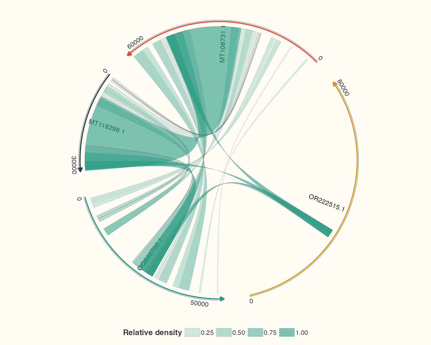
stat_ribbon_density() maps a computed density, and stat_ribbon_bundle() performs its explicit aggregation during build. The ordinary ribbon geom still draws one ribbon per row. Interpret count, reported length and identity weighting in their own units; more opaque ribbons need not mean stronger independently validated homology. A point anchor without direction evidence cannot acquire an aggregate orientation merely because its endpoints are equal.

Choose interval ribbons or point links

After this page’s preparation code:

Code

# Midpoints summarize existing HSPs for display; they are not new alignments.
points <- ribbon_data_example |>
  transmute(
    qaccver, saccver,
    qpos = floor((qstart + qend) / 2),
    spos = floor((sstart + send) / 2),
    pident
  )
p_points <- ggchord(seq_data = seqs) +
  geom_seq() +
  geom_seq_label(size = 4) +
  geom_link_line(aes(link_colour = pident),
    data = points,
    arrow = arrow(length = unit(2, "mm")), linewidth = .7
  ) +
  scale_link_colour_gradientn(
    colours = identity_palette, values = identity_values,
    limits = c(0, 100), breaks = identity_breaks,
    name = "Identity (%)", guide = guide_ggchord_colourbar(
      available_aes = "link_colour",
      position = "bottom", direction = "horizontal",
      theme = doc_legend_theme + theme(legend.key.width = unit(65, "mm"), legend.key.height = unit(5, "mm"))
    )
  ) +
  scale_seq_colour_manual(values = seq_palette) +
  coord_chord() +
  doc_theme
p_points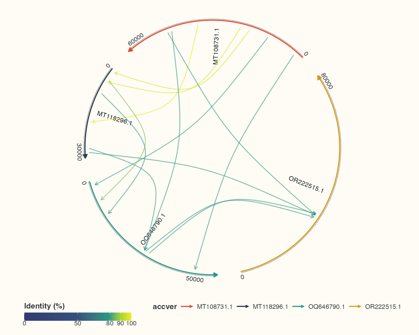

Midpoint links derived from existing HSP intervals · Click to enlarge

Point positions are integer midpoints of real bundled HSPs; identity remains the reported pident. Lines use qpos/spos, not interval ends, and an arrow points from query to subject. The line default avoidance is none; ribbon avoidance is uniform. Global chord rotation belongs to the coordinate system. Pair selection and adjacent-row defaults in linear plots are covered in three modes.

The point-link colour scale supplies available_aes = "link_colour" to its colourbar explicitly. Ordinary ggplot2 colourbars and the wrapper default do not accept every extended role; choose the matching role when making a custom guide.

Check your result

Inspect each report and member rows before reading the plot. Aggregated bands are not new alignments; point links summarize midpoints of existing HSPs.

Continue: Focus, segments and homology →