0.16.6 documentation

Site guide · find your task

Setup and learning paths

HomeInstall and prepare the environmentChoose your learning module

Module I · Chord

1.1 Tables and field meanings1.2 Produce and import comparisons1.3 Build the layers step by step1.4 Direction, curvature and clearance1.5 Filter and summarize links1.6 Full source-file workflow1.7 Complete chord showcase

Module II · Collinear

2.1 Reuse chord input tables2.2 Switch coordinates and add layers2.3 Routes, clearance and the ruler2.4 Compare CDS neighbourhoods2.5 Focus, anchors and segments2.6 Complete collinear showcase

Module III · Plasmid

3.1 DNA, annotations and 13 references3.2 From a circle to annotation layers3.3 Features, primers and restriction3.4 Thirteen plasmid references3.5 Complete plasmid cases

Consult as needed · Data and layers

Prepare tables and coordinatesImport and convert dataImport nucleotide and protein alignmentsProject protein intervals to genomic coordinatesFeatures, stacking and genomic decorationLabels and local placementQuantitative tracksMappings, scales, guides and themesSet values by sequence and strandCommon adjustments and grammarExport, preview and diagnostics

Learning map and reference

Articles and complete workflowsFunction referenceReproducible galleryFrequently asked questionsMigrate to the candidate APITerminology and design sourcesDevelopment status and changes

Features, stacking and genomic decoration

On this page

• Prepare this page
• Preserve feature semantics
• Choose shapes by meaning
• Highlight an interval without rewriting observations
• Check your result

Draw real annotations as independent layers, choose suitable shapes and share stacking positions between overlapping intervals and text.

Prepare this page

In a fresh R session, run the code below, then follow this page in order. Colours and layout are optional display choices; inputs select only the fields needed.

Preparation code — run once on this page

Code

library(ggchord)
library(dplyr)
data(seq_data_example)
data(ribbon_data_example)
data(gene_data_example)
seqs <- seq_data_example |>
  select(accver, length)
links <- ribbon_data_example |>
  select(qaccver, saccver, qstart, qend, sstart, send)
# The fixture preserves biological strands separately from its old display strands.
genes <- gene_data_example |>
  transmute(accver, start, end, strand = source_strand)

# Optional appearance choices; none of these columns or scales is required input.
library(ggchord)
seq_palette <- setNames(
  c("#E64B35", "#233E4A", "#269B82", "#D59B17"),
  c("MT108731.1", "MT118296.1", "OQ646790.1", "OR222515.1")
)
gene_palette <- c("+" = "#CE1536", "-" = "#346B9D", "." = "#8291A6")

library(ggchord)
feature_palette <- c(
  CDS = "#993366", promoter = "#31849B", rep_origin = "#F1E51D",
  primer_bind = "#A020F0", misc_feature = "#A6ACB3", protein_bind = "#31849B"
)

library(ggchord)
doc_background <- "#FFFCF5"
identity_palette <- c("#303B71", "#36537D", "#269B82", "#A5D52C", "#ECEB31")
identity_values <- c(0, 0.5, 0.8, 0.9, 1)
identity_breaks <- c(0, 50, 80, 90, 100)
doc_legend_theme <- theme(
  legend.title = element_text(size = 13, face = "bold"),
  legend.text = element_text(size = 11),
  legend.key.width = unit(9, "mm"), legend.key.height = unit(5, "mm"),
  legend.spacing.x = unit(9, "mm"), legend.spacing.y = unit(7, "mm"),
  legend.margin = margin(l = 4, r = 4, unit = "mm")
)
sequence_guide <- guide_ggchord_legend(nrow = 1, theme = doc_legend_theme)
strand_guide <- guide_ggchord_legend(
  nrow = 1, override.aes = list(strand = c("+", "-")), theme = doc_legend_theme
)
identity_guide <- guide_ggchord_colourbar(
  position = "left", direction = "vertical",
  theme = theme(
    legend.key.height = unit(75, "mm"), legend.key.width = unit(5, "mm"),
    legend.title = element_text(size = 13, face = "bold"),
    legend.text = element_text(size = 11), legend.margin = margin(r = 7, unit = "mm")
  )
)
doc_theme <- theme_ggchord_publication(
  axis.text = element_text(size = 11),
  axis.text.check.overlap = TRUE
) +
  theme(
    legend.position = "bottom",
    legend.title = element_text(size = 13, face = "bold"),
    legend.text = element_text(size = 11),
    legend.key.width = unit(9, "mm"), legend.key.height = unit(5, "mm"),
    legend.spacing.x = unit(9, "mm"), legend.spacing.y = unit(7, "mm"),
    legend.box.spacing = unit(6, "mm"),
    plot.background = element_rect(fill = doc_background, colour = NA),
    panel.background = element_blank(),
    plot.title = element_text(face = "bold", size = 18),
    plot.subtitle = element_text(size = 10, colour = "#5C625A"),
    plot.margin = margin(14, 18, 14, 18)
  )
doc_axis <- function(coordinates = "relative") {
  scale_seq_position_continuous(
    coordinates = coordinates, n.breaks = 3, minor_breaks = NULL,
    labels = function(x) format(x, scientific = FALSE, big.mark = ",", trim = TRUE)
  )
}

library(dplyr)
data(plasmid_example_pUC19)
plasmid_seq <- plasmid_example_pUC19 |>
  select(accver, length)
feature_source <- find_common_features(plasmid_example_pUC19)
features <- feature_source |>
  select(accver, start, end, strand, type, anno)

Preserve feature semantics

The preparation above loads the actual pUC19 annotations; the circular example introduces their roles. This table retains actual overlapping pUC19 annotations and unknown strands. Geometry and fill map separately from the same category; an explicit fixed shape would override shape mapping.

Code

stack_features <- features |>
  select(accver, start, end, strand, type, anno)
stack_position <- position_feature_stack(spacing = .12)
feature_shapes <- setNames(ifelse(names(feature_palette) == "CDS", "arrow", "block"), names(feature_palette))
p_stack <- ggchord(seq_data = plasmid_seq) +
  geom_seq(show.legend = FALSE) +
  geom_feature(aes(feature_fill = type, feature_shape = type),
    data = stack_features,
    width = .08, position = stack_position
  ) +
  geom_feature_label_repel(data = stack_features, position = stack_position, size = 3.8, label_fit = "shrink", label_min_size = 2.8) +
  scale_feature_shape_manual(values = feature_shapes) +
  scale_feature_fill_manual(values = feature_palette) +
  coord_collinear() +
  doc_axis() +
  doc_theme
p_stack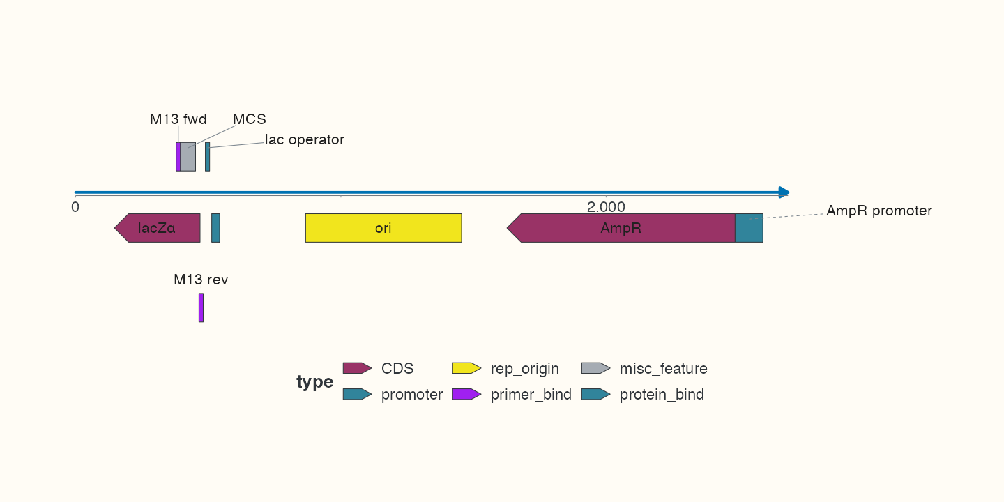

Stacked overlapping annotations from the pUC19 reference · Click to enlarge

position_feature_stack() resolves overlapping annotation lanes. The label layer uses the same Position, so text anchors follow those lanes. Prefer unique feature_id values for subset/reordered label inputs. The strict gene shortcut requires known +/-; general features retain unknown/bidirectional semantics.

Choose shapes by meaning

Geometry	Typical use	Important distinction
arrow, compact_arrow	Directional coding/feature interval	Known direction is evidence, not a display guess
block, capped_line	Region or unfilled interval	Shape choice does not infer biological function
promoter_arrow, primer_arrow, primer_arc	Declared promoter/primer-style annotation	Computational matching and drawing are separate
marker, chevron, lollipop	Custom interval/point-like emphasis	Keep real interval metadata; display shape is a mapping

geom_gene() and geom_feature_plasmid() are useful presets, not aliases with identical defaults. Use position_strand() for signed offsets and position_plasmid() as a circular placement preset; the latter is not a fourth coordinate mode.

Highlight an interval without rewriting observations

Code

regions <- tibble(
  accver = links$qaccver[1], start = min(links$qstart[1], links$qend[1]),
  end = max(links$qstart[1], links$qend[1]), category = "alignment interval"
)
p_decorated <- ggchord(seq_data = seqs, ribbon_data = links) +
  geom_seq_region(aes(region_fill = category), data = regions, colour = NA) +
  geom_link_ribbon(fill = "#6BAFA6", alpha = .4) +
  geom_seq() +
  geom_seq_label(size = 4) +
  scale_region_fill_manual(values = c("alignment interval" = "#F4D35E")) +
  scale_seq_colour_manual(values = seq_palette) +
  geom_seq_scale(length = 10000) +
  coord_collinear() +
  doc_axis() +
  doc_theme
p_decorated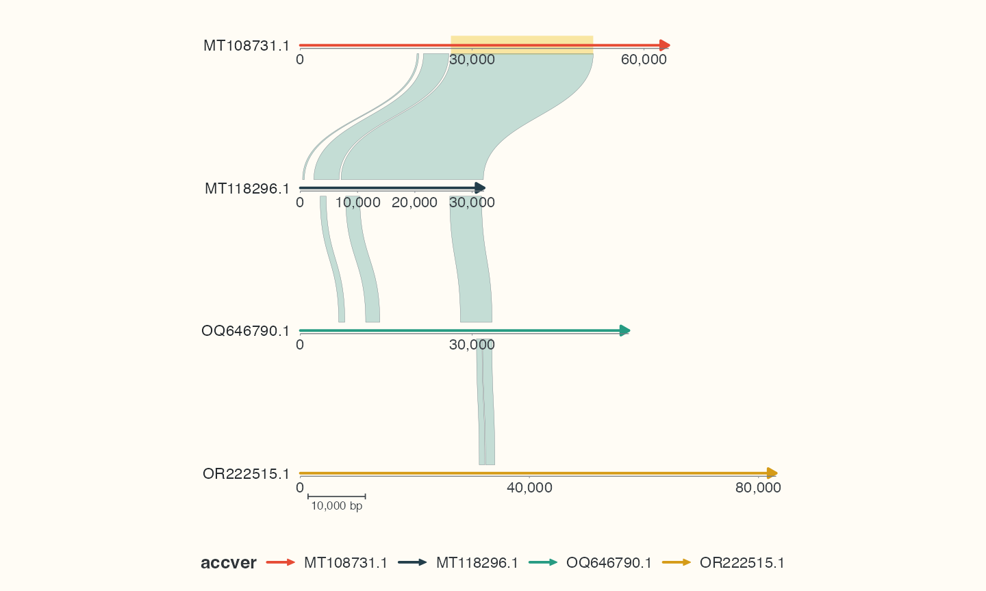

Highlighting the query interval of an observed alignment · Click to enlarge

A region overlay uses its own table and region_fill scale. geom_seq_label() names sequences, geom_seq_center_label() supplies name/length in a single circle, and geom_seq_break() marks cropped/segmented ends. geom_seq_scale() is an independent bp reference bar for collinear plots; it differs from scale_seq_position_continuous(), which controls genomic axes on sequences. An ordinary ggplot2 annotation should use position mapping instead of treating bp as Cartesian x/y.

Check your result

Check intervals and strands before shapes and labels. Unknown strands remain in general features; stacking changes display placement, not genomic coordinates.

Continue: Labels and local placement →