Chapters and reference
Shared techniques · Section 6 of 10
5.5 Scales, guides and themes
On this page
- 1 Independent input and scale responsibilities
- 2 Continuous, stepped and direct colour values
- 3 Identity preserves supplied colour values
- 4 Category fill, opacity, outline and line type
- 5 Independent scales for point links
- 6 Feature, gene and region roles
- 7 Gene strand, sequence rings and regions
- 8 Named track domains and colours
- 9 Guides, spelling aliases and staged mapping
- 10 Themes style non-data appearance
- 11 Selection rules
Choose the meaning of data before roles and scales. Use the same observed HSPs, annotations and GC windows for continuous values, categories, identity, opacity, widths, line types and themes, grouping related helpers on one page.
1 Independent input and scale responsibilities
Independently load ggchord and optional dplyr. Complete lengths, HSP identity and query/subject IDs come from bundled source records. Named vectors assign display values to existing categories, not new samples or measurements. Map inside aes, fix styles in geoms, and let explicit scales override automatic defaults. Explicit fixed aesthetics override matching mappings; omit fixed alpha when mapping opacity.
R · Example code
library(ggchord)
library(dplyr)
scale_seqs <- seq_data_example[c("accver", "length")]
scale_links <- ribbon_data_example
scale_ids <- scale_seqs$accver
scale_colours <- setNames(c("#E64B35", "#233E4A", "#269B82", "#D59B17"), scale_ids)
scale_opacity <- setNames(c(0.35, 0.55, 0.75, 0.95), scale_ids)
scale_lines <- setNames(c("solid", "dashed", "dotted", "dotdash"), scale_ids)
scale_base <- ggchord(scale_seqs, ribbon_data = scale_links) + geom_seq() + coord_chord()
scale_numeric <- scale_base + geom_link_ribbon(aes(ribbon_fill = pident))
2 Continuous, stepped and direct colour values
Both map observed pident to ribbon_fill with fixed 0–100 domain, palette and dimensions. Gradientn interpolates continuously; stepsn uses explicit breaks. Matching colours do not establish new homology. Values place palette anchors, not source pident; breaks control ticks/steps and limits the domain. Check NA and out-of-bounds policy rather than treating missing values as zero.
R · Example code
p_comparescalegradient <- scale_numeric +
  scale_ribbon_fill_gradientn(colours = c("#303B71", "#269B82", "#ECEB31"),
    limits = c(0, 100), breaks = c(0, 50, 80, 90, 95, 100), name = "Identity (%)") +
  guides(ribbon_fill = guide_ggchord_colourbar())
view_ggchord(p_comparescalegradient, width = 9, height = 7, units = "in")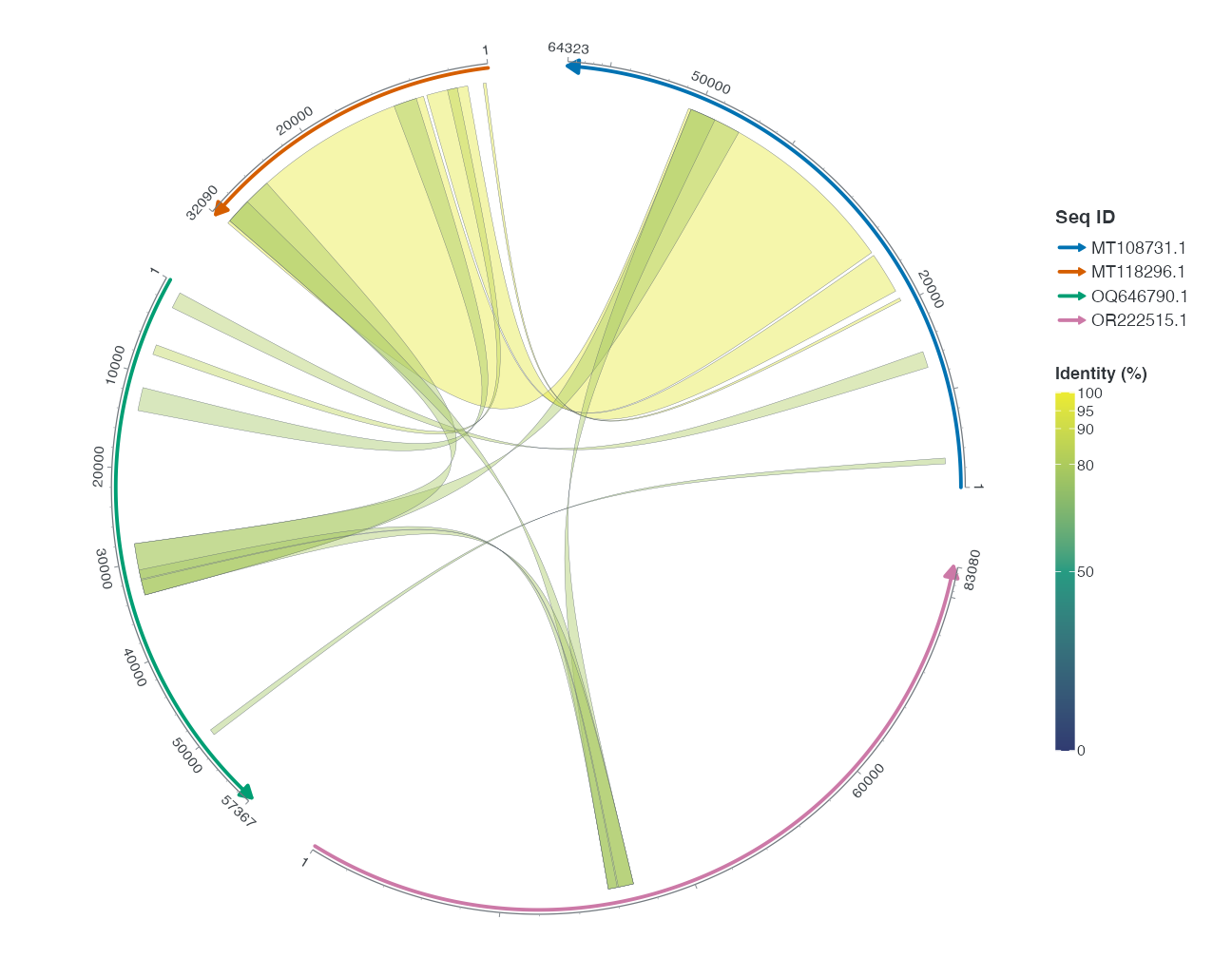
R · Example code
p_comparescalesteps <- scale_numeric +
  scale_ribbon_fill_stepsn(colours = c("#303B71", "#269B82", "#ECEB31"),
    breaks = c(0, 50, 80, 90, 95, 100), limits = c(0, 100),
    name = "Identity (%)", guide = ggplot2::guide_coloursteps(available_aes = "ribbon_fill",
      even.steps = FALSE, show.limits = TRUE, position = "left",
      direction = "vertical", theme = theme(legend.key.height = grid::unit(80, "mm"))))
view_ggchord(p_comparescalesteps, width = 9, height = 7, units = "in")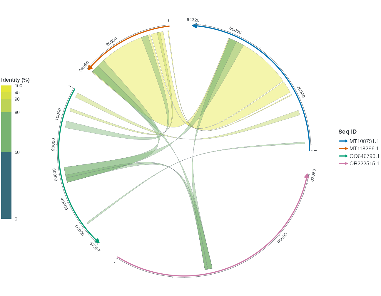
3 Identity preserves supplied colour values
First derive display colours from observed identity using an explicit 90% threshold, then preserve those strings with scale_ribbon_fill_identity. This is declared display classification, not a way to recover continuous identity. Use a gradient for a continuous legend. Identity normally hides its guide; provide deliberate breaks, labels and guide when one is needed.
R · Example code
scale_identity_links <- scale_links |>
  mutate(display_colour = if_else(pident >= 90, "#269B82", "#303B71"))
p_scale_identity <- ggchord(scale_seqs, ribbon_data = scale_identity_links) +
  geom_seq() + geom_link_ribbon(aes(ribbon_fill = display_colour)) +
  scale_ribbon_fill_identity() + coord_chord()
invisible(ggplot2::ggplot_build(p_scale_identity))
4 Category fill, opacity, outline and line type
The same qaccver receives the same display values. Name manual values by actual categories to avoid order-dependent mismatches. This combines independently trained roles rather than claiming a single-parameter visual experiment. Use scale_ribbon_alpha_continuous(range=...) for numeric opacity and scale_ribbon_alpha_manual for categories. Colour and linetype change outlines, not alignment direction.
R · Example code
p_scale_manual <- scale_base +
  geom_link_ribbon(aes(ribbon_fill = qaccver, ribbon_alpha = qaccver,
    ribbon_colour = qaccver, ribbon_linetype = qaccver)) +
  scale_ribbon_fill_manual(values = scale_colours) +
  scale_ribbon_alpha_manual(values = scale_opacity) +
  scale_ribbon_colour_manual(values = scale_colours) +
  scale_ribbon_linetype_manual(values = scale_lines) +
  scale_seq_colour_manual(values = scale_colours) +
  guides(ribbon_fill = guide_ggchord_legend(nrow = 1))
invisible(ggplot2::ggplot_build(p_scale_manual))
5 Independent scales for point links
Explicitly calculate midpoints of observed HSPs; point links do not display full spans. Manual helpers map link_colour, link_alpha, link_linewidth and link_linetype by category; gradientn, alpha_continuous and linewidth_continuous map numeric values. Construct category and numeric combinations separately.
Automatic numeric pident mappings use the 0–100 domain and six Identity ticks: 0, 50, 80, 90, 95 and 100. Explicit scales keep their own settings. The example sets the same domain, ticks and title for all three channels so their legend keys can combine.
R · Example code
scale_points <- scale_links |>
  slice_head(n = 6) |>
  mutate(qpos = floor((qstart + qend) / 2), spos = floor((sstart + send) / 2))
p_scale_linkbase <- ggchord(scale_seqs) + geom_seq() + coord_chord()
R · Example code
p_scale_linkmanual <- p_scale_linkbase +
  geom_link_line(aes(link_colour = saccver, link_alpha = saccver,
    link_linewidth = saccver, link_linetype = saccver), data = scale_points) +
  scale_link_colour_manual(values = scale_colours) +
  scale_link_alpha_manual(values = scale_opacity) +
  scale_link_linewidth_manual(values = setNames(c(0.3, 0.5, 0.7, 0.9), scale_ids)) +
  scale_link_linetype_manual(values = scale_lines)
invisible(ggplot2::ggplot_build(p_scale_linkmanual))
R · Example code
p_comparescalelinkcontinuous <- p_scale_linkbase +
  geom_link_line(aes(link_colour = pident, link_alpha = pident,
    link_linewidth = pident), data = scale_points) +
  scale_link_colour_gradientn(
    colours = c("#303B71", "#ECEB31"), limits = c(0, 100),
    breaks = c(0, 50, 80, 90, 95, 100), name = "Identity (%)",
    guide = guide_ggchord_legend()
  ) +
  scale_link_alpha_continuous(
    range = c(0.3, 0.9), limits = c(0, 100),
    breaks = c(0, 50, 80, 90, 95, 100), name = "Identity (%)"
  ) +
  scale_link_linewidth_continuous(
    range = c(0.2, 1), limits = c(0, 100),
    breaks = c(0, 50, 80, 90, 95, 100), name = "Identity (%)"
  )
view_ggchord(p_comparescalelinkcontinuous, width = 9, height = 7, units = "in")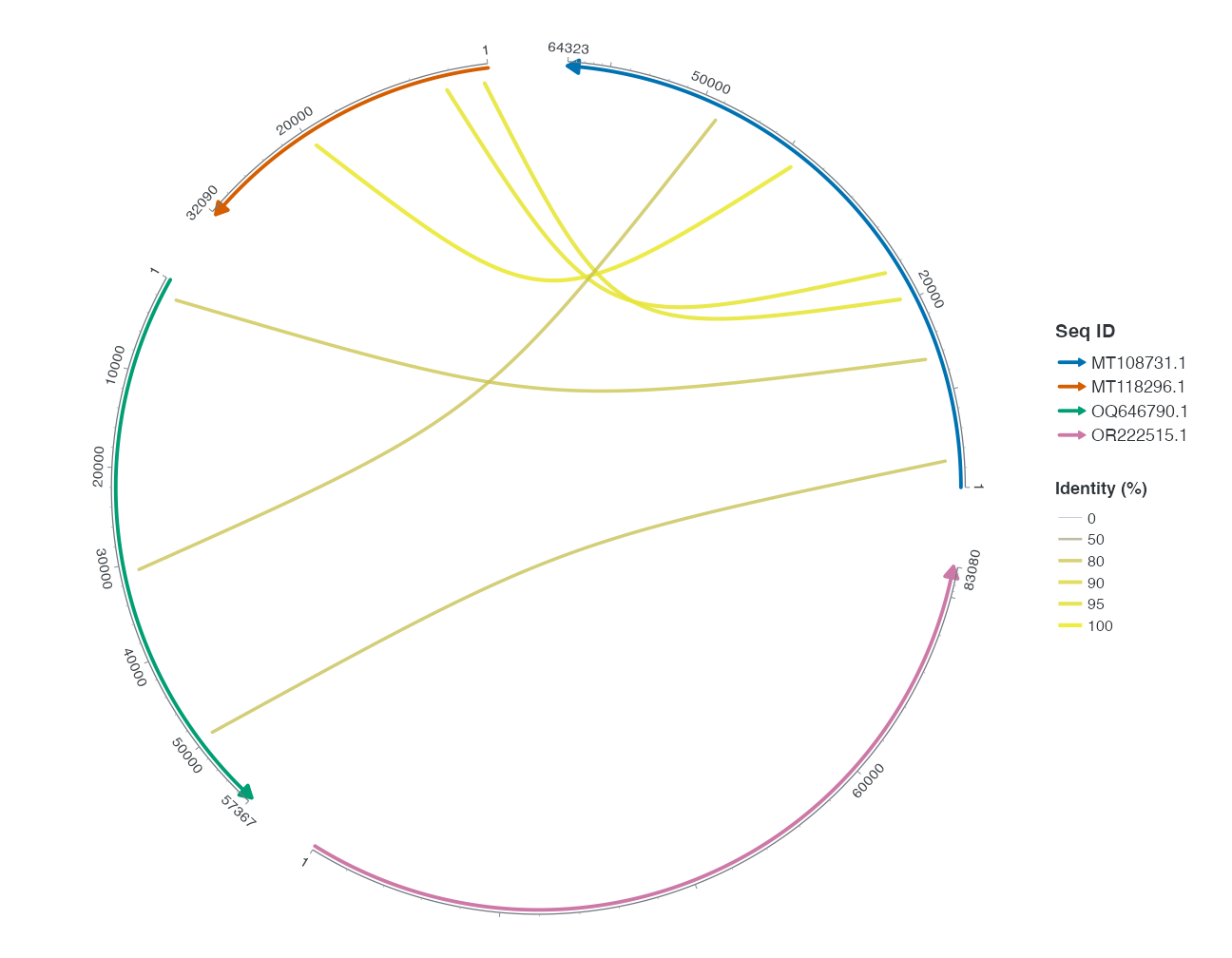
6 Feature, gene and region roles
Map feature_fill and feature_shape to the same type to merge their guide silhouettes; request a separate shape guide explicitly. Fixed shape overrides its mapping. Mapping all types to arrow demonstrates mapping without inventing functional shape semantics. Plasmid fill/shape presets use their documented category rules.
R · Example code
scale_feature_data <- head(find_common_features(plasmid_example_pUC19), 6)
feature_types <- unique(scale_feature_data$type)
feature_colours <- setNames(rep(c("#993366", "#31849B", "#D59B17"),
  length.out = length(feature_types)), feature_types)
p_scale_feature <- ggchord(plasmid_example_pUC19) + geom_seq() +
  geom_feature(aes(feature_fill = type, feature_shape = type), data = scale_feature_data) +
  scale_feature_fill_manual(values = feature_colours) +
  scale_feature_shape_manual(values = setNames(rep("arrow", length(feature_types)), feature_types)) +
  coord_circular()
invisible(ggplot2::ggplot_build(p_scale_feature))
R · Example code
p_scale_preset <- ggchord(plasmid_example_pUC19) + geom_seq() +
  geom_feature(aes(feature_fill = type, feature_shape = type), data = scale_feature_data) +
  scale_feature_fill_plasmid() + scale_feature_shape_plasmid() + coord_circular()
invisible(ggplot2::ggplot_build(p_scale_preset))
7 Gene strand, sequence rings and regions
Restore biological strands from source_strand. Region, gene and ribbon fill roles are independent. seq_ring requires explicit positive radii, never inferred track counts; it conflicts with seq_radius and collinear mode. Sequence radius mapping is distinct from quantitative position_track bands.
R · Example code
scale_gene_data <- gene_data_example |>
  transmute(accver, start, end, strand = source_strand)
p_scale_gene <- ggchord(scale_seqs, gene_data = scale_gene_data) + geom_seq() +
  geom_gene() + scale_gene_fill_manual(values = c("+" = "#CE1536", "-" = "#346B9D")) + coord_chord()
p_scale_ring <- ggchord(scale_seqs) + geom_seq(aes(seq_ring = accver)) +
  scale_seq_ring_manual(values = setNames(c(0.8, 1, 1.2, 1.4), scale_ids)) + coord_chord()
invisible(ggplot2::ggplot_build(p_scale_gene))
invisible(ggplot2::ggplot_build(p_scale_ring))
R · Example code
scale_region_data <- scale_links |>
  slice_head(n = 3) |>
  transmute(accver = qaccver, start = pmin(qstart, qend), end = pmax(qstart, qend))
p_scale_region <- ggchord(scale_seqs) + geom_seq() +
  geom_seq_region(aes(region_fill = accver), data = scale_region_data) +
  scale_region_fill_manual(values = scale_colours) + coord_chord()
invisible(ggplot2::ggplot_build(p_scale_region))
8 Named track domains and colours
Compute windows from actual pUC19 DNA. track_value controls height; track_fill/track_colour train separate colour scales, with IDs matching position_track. The 0.5 threshold is a display choice and full fractions remain. Tiles do not average data; NA heights do not become zero. Declare scales for each ID independently.
R · Example code
plasmid <- plasmid_example_pUC19
track_seq <- plasmid[c("accver", "length")]
starts <- seq.int(1, plasmid$length, by = 100)
bins <- data.frame(accver = plasmid$accver, start = starts,
                   end = pmin(starts + 99, plasmid$length))
bins$gc <- vapply(seq_len(nrow(bins)), function(i) {
  bases <- strsplit(substr(plasmid$sequence, bins$start[i], bins$end[i]), "")[[1]]
  mean(bases %in% c("G", "C"))
}, numeric(1))
head(bins)
R · Example code
scale_track_bins <- bins |>
  mutate(gc_class = if_else(gc >= 0.5, "GC >= 0.5", "GC < 0.5"))
p_scale_trackfill <- ggchord(track_seq) + geom_seq() +
  geom_track_tile(aes(track_fill = gc_class), data = scale_track_bins,
    position = position_track("classes")) +
  scale_track_fill_manual("classes", values = c("GC >= 0.5" = "#31849B", "GC < 0.5" = "#D59B17")) +
  coord_circular()
p_scale_trackcolour <- ggchord(track_seq) + geom_seq() +
  geom_track_tile(aes(track_colour = gc_class), data = scale_track_bins,
    position = position_track("classes"), fill = NA) +
  scale_track_colour_manual("classes", values = c("GC >= 0.5" = "#31849B", "GC < 0.5" = "#D59B17")) +
  coord_circular()
invisible(ggplot2::ggplot_build(p_scale_trackfill))
invisible(ggplot2::ggplot_build(p_scale_trackcolour))
R · Example code
p_scale_trackgradient <- ggchord(track_seq) + geom_seq() +
  geom_track_tile(aes(track_fill = gc, track_colour = gc), data = bins,
    position = position_track("gc")) +
  scale_track_fill_gradientn("gc", colours = c("#D59B17", "#31849B")) +
  scale_track_colour_gradientn("gc", colours = c("#D59B17", "#31849B")) +
  coord_circular()
invisible(ggplot2::ggplot_build(p_scale_trackgradient))
9 Guides, spelling aliases and staged mapping
guide_ggchord_legend manages discrete role guides and guide_ggchord_colourbar continuous colour bars. show.legend controls participation, guides chooses guides, and theme controls position/direction/appearance. Colour/color aliases are equivalent: guide_ggchord_colorbar, scale_seq_color_manual, scale_ribbon_color_manual, scale_link_color_manual and scale_link_color_gradientn correspond to colour versions. Do not add both synonymous scales expecting cumulative control.
after_stat reads computed variables such as bundle_n in the next section; after_scale computes supported visual attributes after scaling. They come from ggplot2 and have distinct staged semantics even when their R objects compare equal. All ggplot2/grid reexports follow upstream help, with ownership explicit in the parameter atlas.
10 Themes style non-data appearance
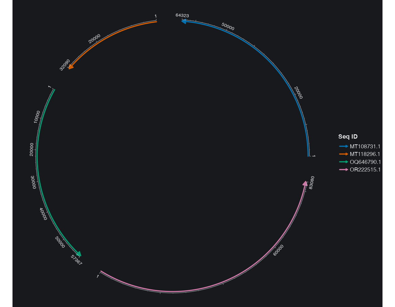
theme_ggchord, minimal, publication and dark are alternative non-data style starting points; plasmid is tailored to single circular maps. Only the theme differs below; sequence data and mappings remain. Axis gaps, tick lengths and text offsets use documented physical units. Theme fields are not accver-keyed geometry lists. Hiding text does not remove sequences.
R · Example code
theme_examples <- list(
  default = theme_ggchord(), minimal = theme_ggchord_minimal(),
  publication = theme_ggchord_publication(), dark = theme_ggchord_dark()
)
for (selected_theme in theme_examples) {
  invisible(ggplot2::ggplot_build(scale_base + selected_theme))
}
p_comparethememinimal <- scale_base + theme_ggchord_minimal()
p_comparethemedark <- scale_base + theme_ggchord_dark()
p_theme_plasmid <- ggchord(plasmid_example_pUC19) + geom_seq() +
  coord_circular() + theme_ggchord_plasmid()
invisible(ggplot2::ggplot_build(p_theme_plasmid))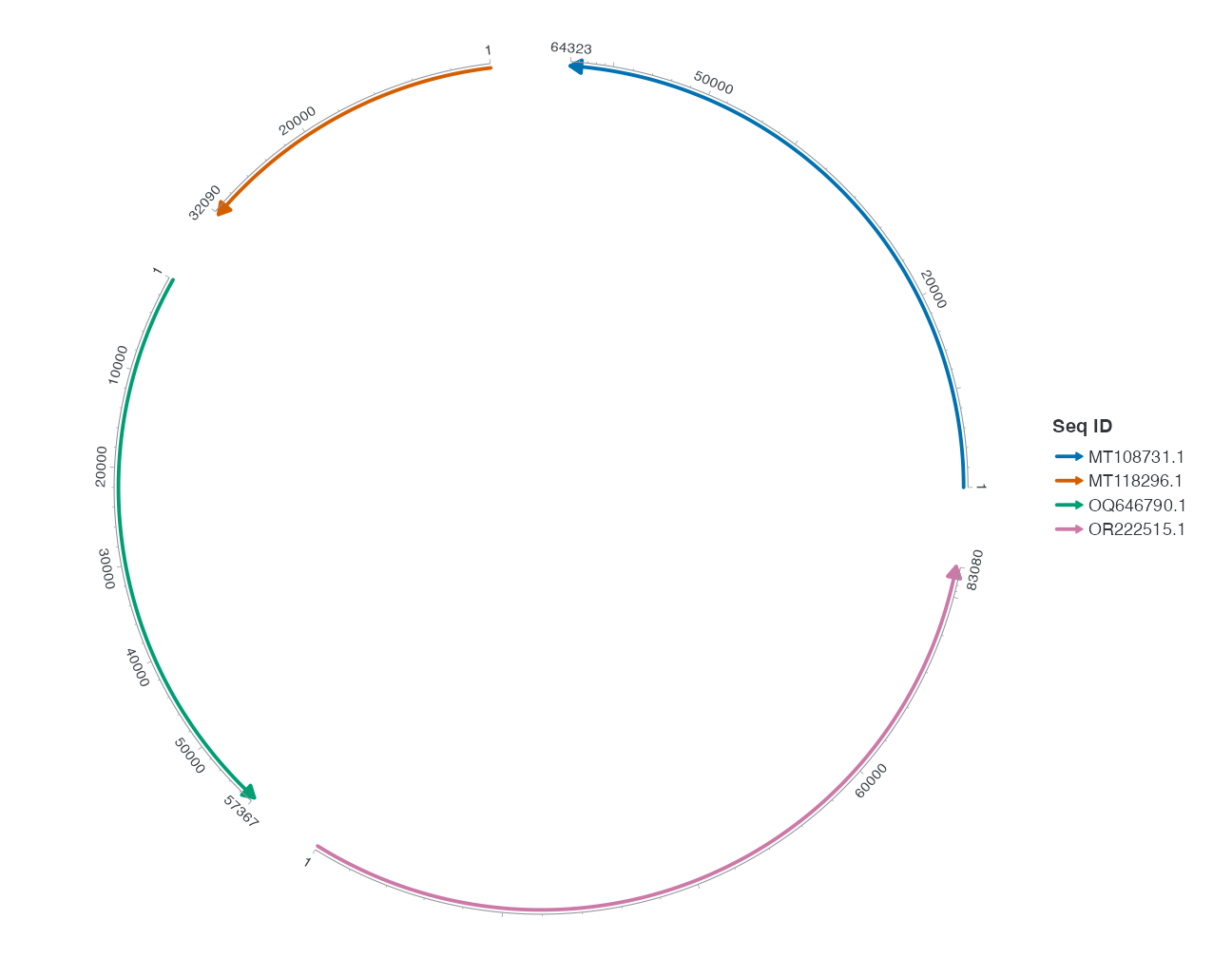
11 Selection rules
Switch pident from gradient to explicit steps, restore the gradient, then change only the alpha output range. Check that guides still represent the same data units. Give additional layers independent data/mapping and retain explicit user scales. See the parameter atlas for complete defaults, types and forwarding, and link statistics for aggregation.