0.16.6 documentation

Site guide · find your task

Setup and learning paths

HomeInstall and prepare the environmentChoose your learning module

Module I · Chord

1.1 Tables and field meanings1.2 Produce and import comparisons1.3 Build the layers step by step1.4 Direction, curvature and clearance1.5 Filter and summarize links1.6 Full source-file workflow1.7 Complete chord showcase

Module II · Collinear

2.1 Reuse chord input tables2.2 Switch coordinates and add layers2.3 Routes, clearance and the ruler2.4 Compare CDS neighbourhoods2.5 Focus, anchors and segments2.6 Complete collinear showcase

Module III · Plasmid

3.1 DNA, annotations and 13 references3.2 From a circle to annotation layers3.3 Features, primers and restriction3.4 Thirteen plasmid references3.5 Complete plasmid cases

Consult as needed · Data and layers

Prepare tables and coordinatesImport and convert dataImport nucleotide and protein alignmentsProject protein intervals to genomic coordinatesFeatures, stacking and genomic decorationLabels and local placementQuantitative tracksMappings, scales, guides and themesSet values by sequence and strandCommon adjustments and grammarExport, preview and diagnostics

Learning map and reference

Articles and complete workflowsFunction referenceReproducible galleryFrequently asked questionsMigrate to the candidate APITerminology and design sourcesDevelopment status and changes

Choose your learning module

On this page

• Which view should you choose?
• Prepare this page
• Chord: compare multiple sequences
• Collinear: align local comparisons
• Circular: annotate one sequence
• Check your result

Choose a layout for your question. The examples below compare three views using source-backed bundled records.

Which view should you choose?

Task	Preferred view	Avoid this misreading
Overall relationships among several sequences	Chord	Crossings alone are not evidence of inversion
Annotations on one plasmid or circular sequence	Circular	Multiple sequences do not fit a single-sequence coordinate
Positions, gene order and local neighbourhoods	Collinear	Display alignment or flipping is not a biological conclusion

All three consume existing data; none computes a new BLAST alignment. Try the minimal combinations below, then follow the raw-record workflow, complete plasmid map or local homolog comparison.

Prepare this page

In a fresh R session, run the code below, then follow this page in order. Colours and layout are optional display choices; inputs select only the fields needed.

Preparation code — run once on this page

Code

library(ggchord)
library(dplyr)
data(seq_data_example)
data(ribbon_data_example)
data(gene_data_example)
seqs <- seq_data_example |>
  select(accver, length)
links <- ribbon_data_example |>
  select(qaccver, saccver, qstart, qend, sstart, send)
# The fixture preserves biological strands separately from its old display strands.
genes <- gene_data_example |>
  transmute(accver, start, end, strand = source_strand)

# Optional appearance choices; none of these columns or scales is required input.
library(ggchord)
seq_palette <- setNames(
  c("#E64B35", "#233E4A", "#269B82", "#D59B17"),
  c("MT108731.1", "MT118296.1", "OQ646790.1", "OR222515.1")
)
gene_palette <- c("+" = "#CE1536", "-" = "#346B9D", "." = "#8291A6")

library(ggchord)
feature_palette <- c(
  CDS = "#993366", promoter = "#31849B", rep_origin = "#F1E51D",
  primer_bind = "#A020F0", misc_feature = "#A6ACB3", protein_bind = "#31849B"
)

library(ggchord)
doc_background <- "#FFFCF5"
identity_palette <- c("#303B71", "#36537D", "#269B82", "#A5D52C", "#ECEB31")
identity_values <- c(0, 0.5, 0.8, 0.9, 1)
identity_breaks <- c(0, 50, 80, 90, 100)
doc_legend_theme <- theme(
  legend.title = element_text(size = 13, face = "bold"),
  legend.text = element_text(size = 11),
  legend.key.width = unit(9, "mm"), legend.key.height = unit(5, "mm"),
  legend.spacing.x = unit(9, "mm"), legend.spacing.y = unit(7, "mm"),
  legend.margin = margin(l = 4, r = 4, unit = "mm")
)
sequence_guide <- guide_ggchord_legend(nrow = 1, theme = doc_legend_theme)
strand_guide <- guide_ggchord_legend(
  nrow = 1, override.aes = list(strand = c("+", "-")), theme = doc_legend_theme
)
identity_guide <- guide_ggchord_colourbar(
  position = "left", direction = "vertical",
  theme = theme(
    legend.key.height = unit(75, "mm"), legend.key.width = unit(5, "mm"),
    legend.title = element_text(size = 13, face = "bold"),
    legend.text = element_text(size = 11), legend.margin = margin(r = 7, unit = "mm")
  )
)
doc_theme <- theme_ggchord_publication(
  axis.text = element_text(size = 11),
  axis.text.check.overlap = TRUE
) +
  theme(
    legend.position = "bottom",
    legend.title = element_text(size = 13, face = "bold"),
    legend.text = element_text(size = 11),
    legend.key.width = unit(9, "mm"), legend.key.height = unit(5, "mm"),
    legend.spacing.x = unit(9, "mm"), legend.spacing.y = unit(7, "mm"),
    legend.box.spacing = unit(6, "mm"),
    plot.background = element_rect(fill = doc_background, colour = NA),
    panel.background = element_blank(),
    plot.title = element_text(face = "bold", size = 18),
    plot.subtitle = element_text(size = 10, colour = "#5C625A"),
    plot.margin = margin(14, 18, 14, 18)
  )
doc_axis <- function(coordinates = "relative") {
  scale_seq_position_continuous(
    coordinates = coordinates, n.breaks = 3, minor_breaks = NULL,
    labels = function(x) format(x, scientific = FALSE, big.mark = ",", trim = TRUE)
  )
}

library(dplyr)
data(plasmid_example_pUC19)
plasmid_seq <- plasmid_example_pUC19 |>
  select(accver, length)
feature_source <- find_common_features(plasmid_example_pUC19)
features <- feature_source |>
  select(accver, start, end, strand, type, anno)

Run the preparation above once. Each object below is a normal composable ggplot; print it or use ggsave().

Chord: compare multiple sequences

Code

p_chord <- ggchord(seq_data = seqs, ribbon_data = links, gene_data = genes) +
  geom_link_ribbon(aes(ribbon_fill = qaccver), alpha = .7) +
  scale_ribbon_fill_manual(values = seq_palette, guide = "none") +
  geom_seq(show.legend = FALSE) +
  geom_gene(position = position_strand(.1), width = .04) +
  geom_seq_label(size = 4, seq_label_radius = .84, seq_label_hjust = .5) +
  coord_chord() +
  scale_seq_colour_manual(values = seq_palette) +
  scale_gene_fill_manual(values = gene_palette) +
  doc_theme
p_chord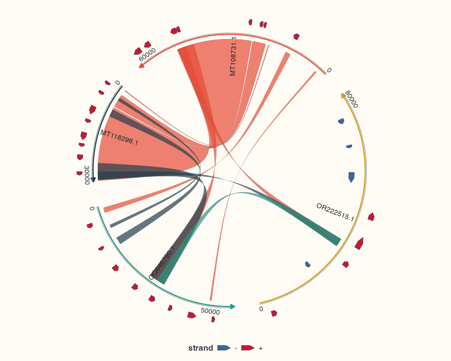

Bundled sequences and alignment intervals in a chord view · Click to enlarge

Links are coloured by query sequence ID using the backbone category palette; this does not encode identity or homolog groups. See the raw-record workflow for colour mapped to reported identity. coord_chord() controls global rotation and fitting. Sequence-local radius, curvature, gap and orientation belong to geom_seq(). A NULL link control point uses the historical origin-based chord route; it does not mean a universal straight link. Ribbon avoidance defaults to uniform, line avoidance to none.

Collinear: align local comparisons

Code

anchors <- genes |>
  group_by(accver) |>
  slice_max(end - start, n = 1, with_ties = FALSE) |>
  ungroup() |>
  select(accver, start, end)
p_collinear <- ggchord(seq_data = seqs, ribbon_data = links, gene_data = genes) +
  geom_link_ribbon(aes(ribbon_fill = qaccver), alpha = .7) +
  scale_ribbon_fill_manual(values = seq_palette, guide = "none") +
  geom_seq() +
  geom_gene(position = position_strand(.1)) +
  geom_seq_label(size = 4) +
  coord_collinear(anchor = anchors, align = "center", orientation = "auto") +
  doc_axis() +
  scale_seq_colour_manual(values = seq_palette) +
  scale_gene_fill_manual(values = gene_palette) +
  doc_theme
p_collinear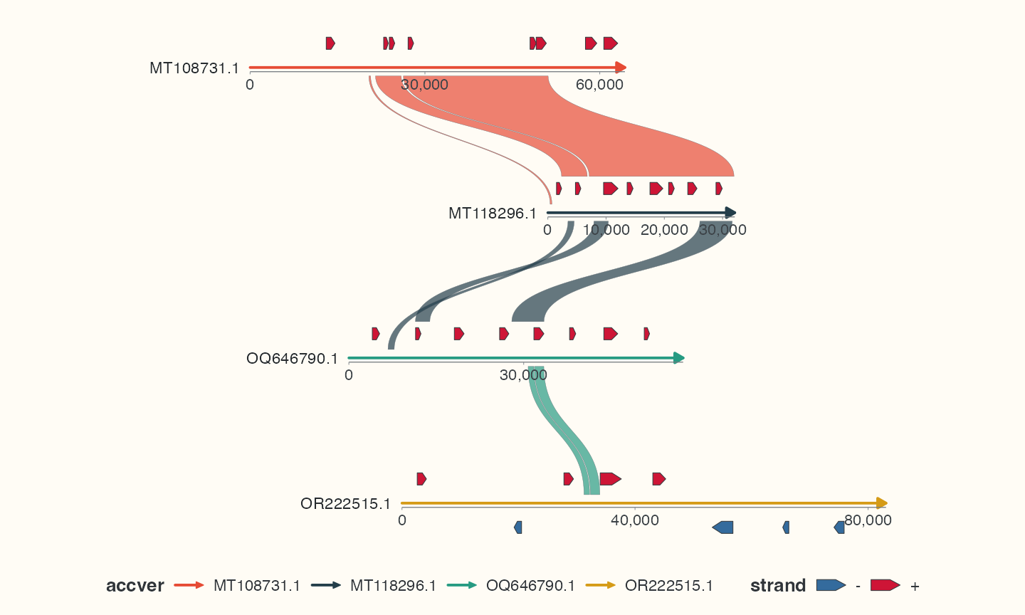

Bundled records aligned to explicitly selected annotation anchors · Click to enlarge

Each sequence is anchored to its own longest known gene for display; this does not assert homology. anchor aligns specified intervals; orientation = "auto" chooses supported orientations using available evidence. Inspect orientation diagnostics rather than assuming biological inversion. Ribbons connect adjacent displayed rows by default; use adjacent_only = FALSE or explicit pairs to retain others. Non-adjacent outlines default to dashed; explicit styles take priority. These rules differ from chord mode. Focus and segments preserve source coordinates for cropped or locally reversed views.

Circular: annotate one sequence

Code

circle_features <- features |>
  filter(type %in% c("CDS", "rep_origin"))
p_circular <- ggchord(seq_data = plasmid_seq) +
  geom_seq() +
  geom_feature(aes(feature_fill = type), data = circle_features, position = position_plasmid()) +
  geom_feature_label_repel(data = circle_features, position = position_plasmid(), size = 4) +
  geom_seq_center_label() +
  scale_feature_fill_manual(values = feature_palette, breaks = unique(circle_features$type)) +
  coord_circular() +
  doc_theme
p_circular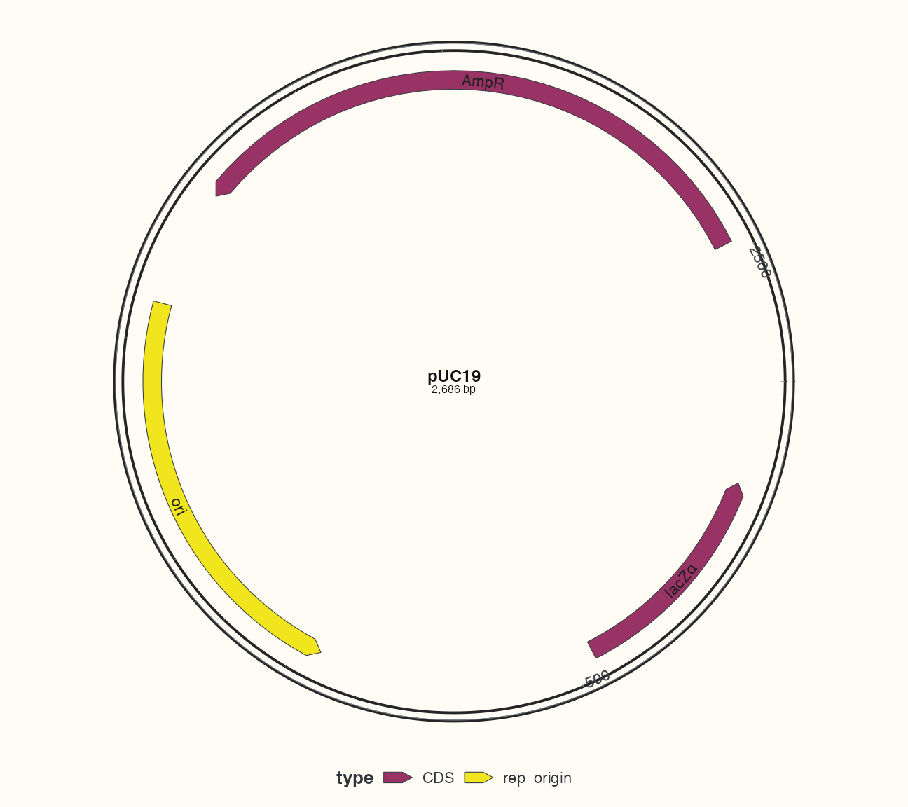

pUC19 annotations in a circular map · Click to enlarge

This example selects CDS and the replication origin for display, retaining the full sequence bp axis. coord_circular() requires a single sequence. General features can carry unknown strand. geom_feature_plasmid() is a convenience preset with its own defaults; choose it explicitly when those defaults fit the task. Primer and restriction layers are described in recognition.

Check your result

First count sequences: use circular for one annotated sequence, chord for the overall link pattern, and collinear for positions, distances or neighbourhoods.

Continue: Get started: your first plot →