Chapters and reference
Shared techniques · Section 8 of 10
5.7 Counts, bins and track statistics
On this page
Data preparation and settings (expand)
R · Example code
plasmid <- plasmid_example_pUC19
track_seq <- plasmid[c("accver", "length")]
starts <- seq.int(1, plasmid$length, by = 100)
bins <- data.frame(accver = plasmid$accver, start = starts,
                   end = pmin(starts + 99, plasmid$length))
bins$gc <- vapply(seq_len(nrow(bins)), function(i) {
  bases <- strsplit(substr(plasmid$sequence, bins$start[i], bins$end[i]), "")[[1]]
  mean(bases %in% c("G", "C"))
}, numeric(1))
head(bins)
R · Example code
library(dplyr)
foundation_source <- ribbon_data_example |>
  mutate(source_hsp_id = paste0("bundled:", row_number()))
foundation_pair <- foundation_source |>
  slice_head(n = 1) |>
  select(qaccver, saccver)
foundation_ids <- c(foundation_pair$qaccver, foundation_pair$saccver)
foundation_seqs <- seq_data_example |>
  filter(accver %in% foundation_ids) |>
  select(accver, length)
foundation_hsp <- foundation_source |>
  filter(qaccver %in% foundation_ids, saccver %in% foundation_ids,
    qaccver != saccver)
foundation_features <- gene_data_example |>
  filter(accver %in% foundation_ids) |>
  transmute(accver, start, end, strand = source_strand, anno)
1 Count observations or display supplied values
bar counts observations at source positions; col displays supplied values. Each accession/window computes its Stat and data Position before view projection or display replication. track=position_track(...) selects the physical band; position independently selects a native data adjustment such as stack or dodge. The earlier position=position_track(...) band spelling remains accepted.
R · Example code
foundation_events <- foundation_hsp |>
  transmute(accver = qaccver, pos = qstart)
p_foundationcount <- ggchord(foundation_seqs) +
  geom_seq() +
  geom_track(
    aes(x = pos), data = foundation_events,
    geom = "bar", track = position_track("query_starts")
  ) +
  coord_collinear()
view_ggchord(p_foundationcount, width = 9, height = 5, units = "in")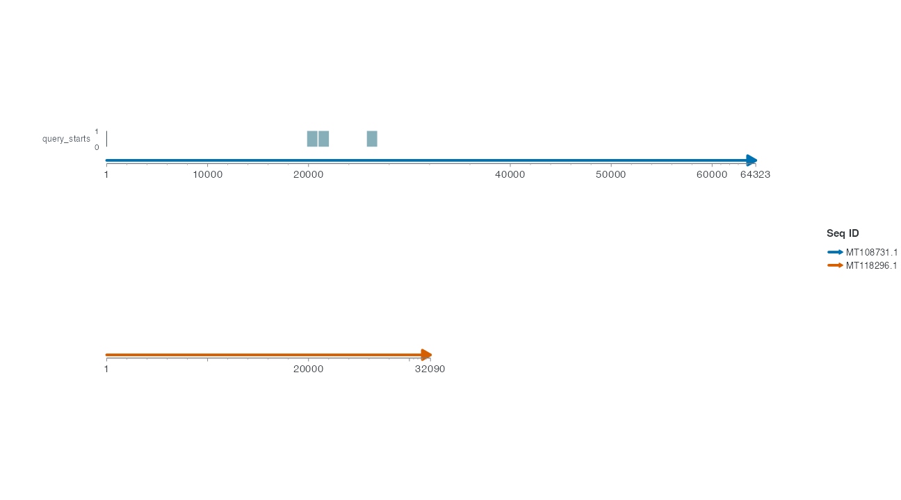
The shortcut below counts the same observations using the same physical band.
R · Example code
p_count_shortcut <- ggchord(foundation_seqs) +
  geom_seq() +
  geom_track_bar(
    aes(x = pos), data = foundation_events,
    track = position_track("query_starts")
  ) +
coord_collinear()| Geometry | Default Stat | Input meaning |
|---|---|---|
| bar | count | x/pos observations, optional weight |
| col | identity | supplied y/track_value; interval or position |
| point, line, path, step, text | identity | source x and local y; text requires label |
| tile, rect, area, ribbon, segment, linerange, errorbar | identity | corresponding native ggplot2 extents |
Available statistics are identity/count/bin/summary, plus the documented smooth/density/ecdf estimation combinations. Bin needs explicit binwidth or breaks. Native group and after_stat mappings are supported; numerical axes retain the statistic’s value units. Arbitrary third-party Geom/Stat plugins and unsupported combinations are rejected. Existing track line/tile shortcuts retain their documented behaviour.
Source position uses x orientation; native text size currently uses mm and polygon outlines are full. Other orientations/size units/partial outlines fail explicitly. Native text styles and path arrows are forwarded.
Native tracks currently require one panel and a ggchord coordinate system. Facets, coord_flip(), raster, boxplot and violin are outside this first supported set and are rejected explicitly. Use coord_collinear(seq_axis = "vertical") for vertical projection. Statistical source membership is preserved before dodge or other data positions. Rectangles and tiles use their supplied bounds without an artificial zero baseline.
2 Two independent bands and display order
Encode the same GC by bar height and colour using explicit gc_height/gc_colour IDs. Set height and colour domains 0–1 separately, with distinct physical widths. The second figure changes only colour order from 2 to 0, moving that band nearer the backbone. Order is a finite priority, not a measurement or required one-based index; ties use IDs. Layers sharing an ID must agree on side/order/width/gap. Lines do not implicitly bridge independent windows.
R · Example code
make_gc_tracks <- function(colour_order) {
  ggchord(track_seq) + geom_seq() +
    geom_track_col(aes(track_value = gc), data = bins,
      position = position_track("gc_height", order = 1, width = grid::unit(8, "mm"))) +
    geom_track_tile(aes(track_fill = gc), data = bins,
      position = position_track("gc_colour", order = colour_order, width = grid::unit(4, "mm"))) +
    scale_track_value_continuous("gc_height", limits = c(0, 1), unit = "GC fraction") +
    scale_track_fill_gradientn("gc_colour", colours = c("#F1E51D", "#31849B"), limits = c(0, 1)) +
    coord_circular()
}
R · Example code
p_comparetracktwo <- make_gc_tracks(colour_order = 2)
view_ggchord(p_comparetracktwo, width = 9, height = 8, units = "in")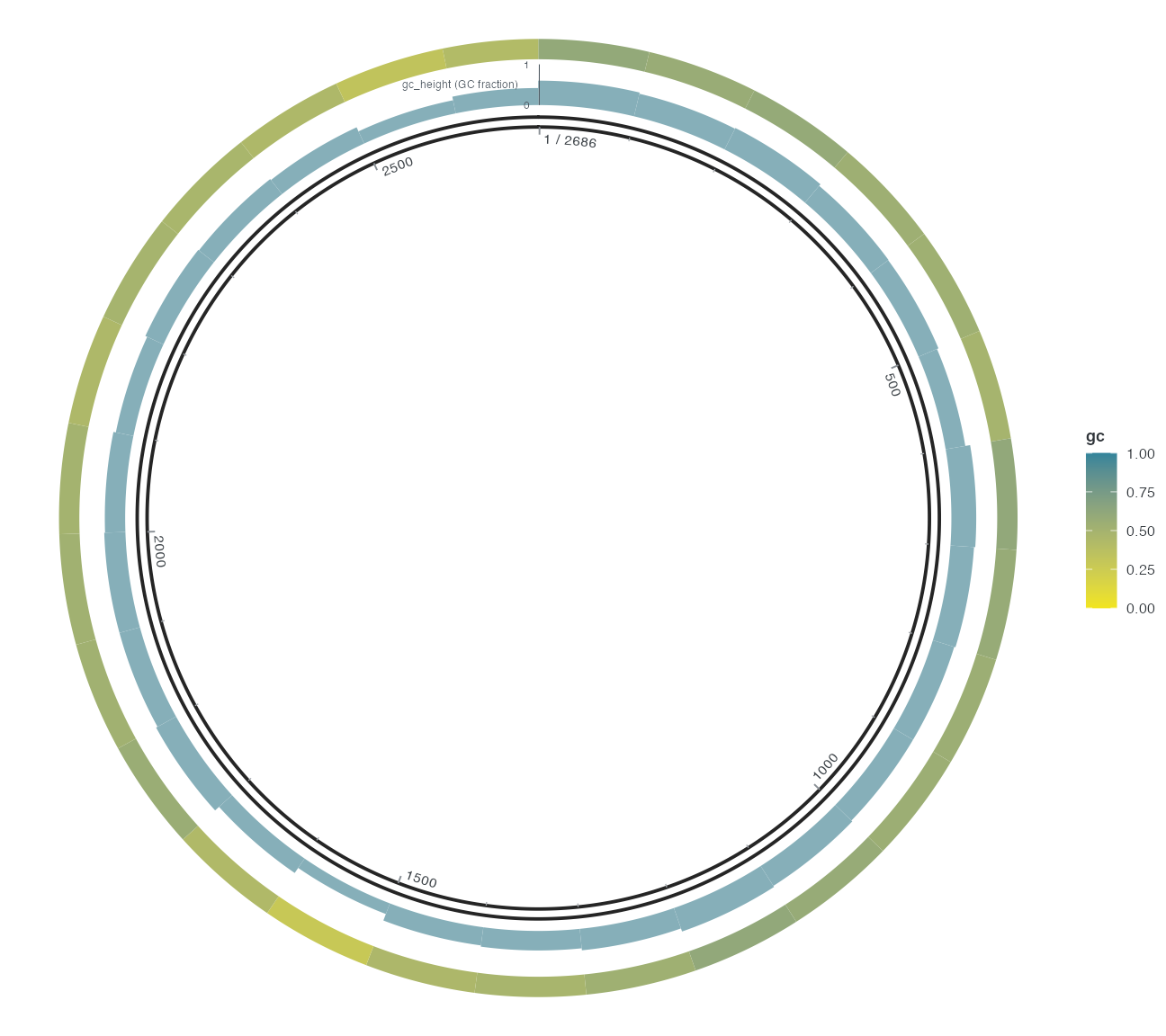
R · Example code
p_comparetrackorder <- make_gc_tracks(colour_order = 0)
view_ggchord(p_comparetrackorder, width = 9, height = 8, units = "in")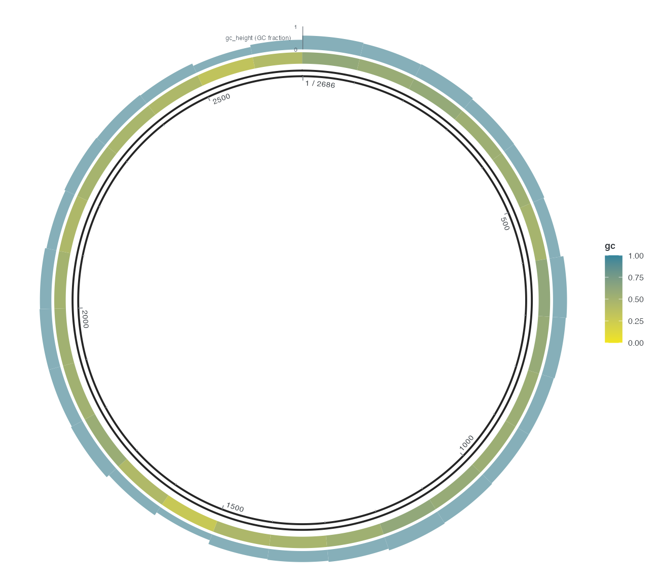
3 DNA windows and line boundaries
GC here is mean(bases %in% c("G", "C")): ambiguous bases remain in the denominator and contribute zero to the numerator. The final window uses its actual number of bases. This pUC19 input has no ambiguous bases; for other inputs explicitly choose and report a policy rather than assuming they are omitted. Focusing clips intervals and retains the original summary; it does not recompute GC for a shortened window. Line tracks connect the supplied samples within their grouping; closed explicitly controls circular closure and gap belongs to physical track placement. Do not use a closed line to imply continuity across omitted source windows.
4 Native source-space estimates
geom_track() also delegates smooth, density and ecdf to native ggplot2 statistics before projection. These create estimates of supplied observations, not additional observations. They run independently by accession/window and explicit group. Estimation source_rows records the eligible group submitted to the estimator after native missing-value handling; it is not per-point influence, positive read support or a custom model’s additional internal filtering report.
| Statistic | Documented geometry | Input and explicit choices | Data Position |
|---|---|---|---|
smooth |
line, path, point, ribbon
|
Source x and raw numerical y; choose method/formula; ribbon requires SE bounds |
"identity" or native PositionIdentity |
density |
line, path, point, area
|
Positions in x, optional weights; choose bandwidth; after_stat(density) is density per source-position unit |
"identity" or native PositionIdentity |
ecdf |
line, path, point, step
|
Positions in x; after_stat(ecdf) is cumulative fraction; explicit pad = FALSE avoids infinite source anchors |
"identity" or native PositionIdentity |
Other combinations of these statistics fail explicitly. Use position = "identity" explicitly for density area because area otherwise defaults to stacking. bounds remains the Track source-boundary policy and does not forward the native density boundary-correction parameter. Facets, boxplots, violins, raster and arbitrary third-party Geom/Stat objects remain unsupported; a numerical name in a function is not a projection contract.
Reuse the real bins and track_seq prepared above. This explicit linear fit is a display summary of the GC fractions, with a native confidence ribbon and mean line sharing one Track:
R · Example code
estimate_bins <- bins |> dplyr::mutate(pos = (start + end) / 2)
estimate_band <- position_track("gc_fit", width = unit(12, "mm"))
p_estimate <- ggchord(track_seq) +
  geom_seq() +
  geom_track(
    aes(x = pos, y = gc), data = estimate_bins, geom = "ribbon", stat = "smooth",
    method = "lm", formula = y ~ x, se = TRUE, position = "identity",
    fill = "#387D88", alpha = 0.2, track = estimate_band
  ) +
  geom_track(
    aes(x = pos, y = gc), data = estimate_bins, geom = "line", stat = "smooth",
    method = "lm", formula = y ~ x, se = FALSE, colour = "#285B65", track = estimate_band
  ) +
  scale_track_value_continuous("gc_fit", name = "GC fit", unit = "fraction") +
  coord_collinear()
view_ggchord(p_estimate)
Statistical fitting uses raw supplied source x/y. A later transformed Track value scale maps the estimates; it does not silently refit a log-space model, unlike placing a transform before a Stat in a native ggplot. If transformed-space fitting is intended, prepare and name that transformed variable explicitly and state its unit. Kernel density of event positions is not measured sequencing depth. ECDF output is a cumulative distribution, not a basewise alignment.
The directed source-backed checks compare native ggplot2 results and group membership for real pUC19 GC windows and G/C positions, plus curved/vertical projection and an explicitly missing-value control. check-track-estimates.R retains the numerical report and actual CI/mean image. Finite source bounds and physical-band constraints still apply; automatic placement does not change the fitted model or manufacture observations.
5 Tracks and windows share source coordinates
Focus pUC19 to 500–1500 bp and trim the same observed GC windows as intervals. focus_ggchord_track does not recompute averages, invent boundary samples or bridge omitted windows. Return to actual DNA and declare new windows/denominators if finer GC summaries are needed.
R · Example code
track_loci <- data.frame(accver = track_seq$accver, start = 500, end = 1500)
focused_bins <- focus_ggchord_track(bins, track_seq, track_loci, type = "interval")
head(focused_bins)
Output / text
  accver start end   gc .source_accver .source_row .source_origin .source_start .source_end .truncated_left .truncated_right
1  pUC19     1   1 0.53          pUC19           5            500           401         500            TRUE            FALSE
2  pUC19     2 101 0.49          pUC19           6            500           501         600           FALSE            FALSE
3  pUC19   102 201 0.61          pUC19           7            500           601         700           FALSE            FALSE
4  pUC19   202 301 0.58          pUC19           8            500           701         800           FALSE            FALSE