Site guide · find your task
Mappings, scales, guides and themes
On this page
Give colours a clear meaning: identify categories or continuous quantities, then choose mappings, scales and guides. Website accents do not dictate data colours.
Prepare this page
In a fresh R session, run the code below, then follow this page in order. Colours and layout are optional display choices; inputs select only the fields needed.
Preparation code — run once on this page
Code
library(ggchord)
library(dplyr)
data(seq_data_example)
data(ribbon_data_example)
data(gene_data_example)
seqs <- seq_data_example |>
  select(accver, length)
links <- ribbon_data_example |>
  select(qaccver, saccver, qstart, qend, sstart, send)
# The fixture preserves biological strands separately from its old display strands.
genes <- gene_data_example |>
  transmute(accver, start, end, strand = source_strand)

# Optional appearance choices; none of these columns or scales is required input.
library(ggchord)
seq_palette <- setNames(
  c("#E64B35", "#233E4A", "#269B82", "#D59B17"),
  c("MT108731.1", "MT118296.1", "OQ646790.1", "OR222515.1")
)
gene_palette <- c("+" = "#CE1536", "-" = "#346B9D", "." = "#8291A6")

library(ggchord)
doc_background <- "#FFFCF5"
identity_palette <- c("#303B71", "#36537D", "#269B82", "#A5D52C", "#ECEB31")
identity_values <- c(0, 0.5, 0.8, 0.9, 1)
identity_breaks <- c(0, 50, 80, 90, 100)
doc_legend_theme <- theme(
  legend.title = element_text(size = 13, face = "bold"),
  legend.text = element_text(size = 11),
  legend.key.width = unit(9, "mm"), legend.key.height = unit(5, "mm"),
  legend.spacing.x = unit(9, "mm"), legend.spacing.y = unit(7, "mm"),
  legend.margin = margin(l = 4, r = 4, unit = "mm")
)
sequence_guide <- guide_ggchord_legend(nrow = 1, theme = doc_legend_theme)
strand_guide <- guide_ggchord_legend(
  nrow = 1, override.aes = list(strand = c("+", "-")), theme = doc_legend_theme
)
identity_guide <- guide_ggchord_colourbar(
  position = "left", direction = "vertical",
  theme = theme(
    legend.key.height = unit(75, "mm"), legend.key.width = unit(5, "mm"),
    legend.title = element_text(size = 13, face = "bold"),
    legend.text = element_text(size = 11), legend.margin = margin(r = 7, unit = "mm")
  )
)
doc_theme <- theme_ggchord_publication(
  axis.text = element_text(size = 11),
  axis.text.check.overlap = TRUE
) +
  theme(
    legend.position = "bottom",
    legend.title = element_text(size = 13, face = "bold"),
    legend.text = element_text(size = 11),
    legend.key.width = unit(9, "mm"), legend.key.height = unit(5, "mm"),
    legend.spacing.x = unit(9, "mm"), legend.spacing.y = unit(7, "mm"),
    legend.box.spacing = unit(6, "mm"),
    plot.background = element_rect(fill = doc_background, colour = NA),
    panel.background = element_blank(),
    plot.title = element_text(face = "bold", size = 18),
    plot.subtitle = element_text(size = 10, colour = "#5C625A"),
    plot.margin = margin(14, 18, 14, 18)
  )
doc_axis <- function(coordinates = "relative") {
  scale_seq_position_continuous(
    coordinates = coordinates, n.breaks = 3, minor_breaks = NULL,
    labels = function(x) format(x, scientific = FALSE, big.mark = ",", trim = TRUE)
  )
}
Build styles from data roles
The preparation above declares the inputs and shared appearance. The example declares categories explicitly: ribbon fill maps query ID; sequence colour maps sequence ID; gene fill maps strand. Manual scale names match those values exactly.
Code
p_styled <- ggchord(seq_data = seqs, ribbon_data = links, gene_data = genes) +
  geom_seq() +
  geom_link_ribbon(aes(ribbon_fill = qaccver), alpha = .5) +
  geom_gene() +
  geom_seq_label(size = 4) +
  coord_collinear() +
  doc_axis() +
  scale_seq_colour_manual(values = seq_palette) +
  scale_gene_fill_manual(values = gene_palette) +
  scale_ribbon_fill_manual(values = seq_palette) +
  guides(gene_fill = guide_ggchord_legend(nrow = 1, theme = doc_legend_theme)) +
  doc_theme
theme_variants <- list(minimal = theme_ggchord_minimal(), dark = theme_ggchord_dark(), plasmid = theme_ggchord_plasmid())
p_styled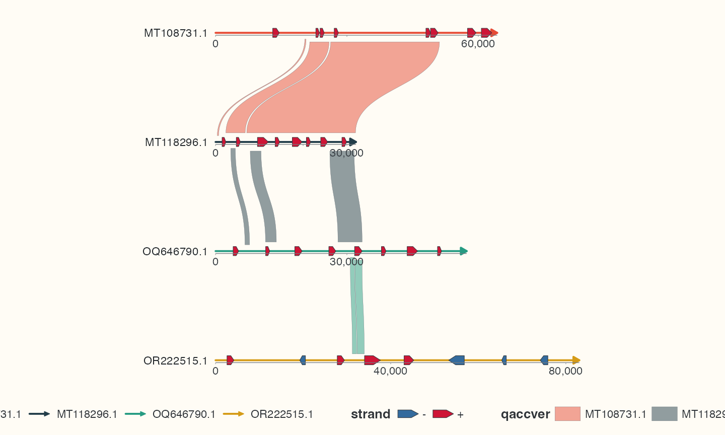
| Role | Mapped data | Useful scale family |
|---|---|---|
seq_colour, seq_ring
|
Sequence/category | Sequence colour or ring manual scales |
ribbon_fill, ribbon_alpha, ribbon_colour, ribbon_linetype
|
Alignment metadata or statistics | Manual, gradient/steps/identity and alpha scales |
feature_fill, feature_shape, gene_fill, region_fill
|
Annotation category or strand | Role-specific manual/preset scales |
link_colour, link_alpha, link_linewidth, link_linetype
|
Point-link metadata | Continuous or manual link scales |
track_value, track_fill, track_colour
|
Values/categories in one named track | Named value domain and colour/fill scales |
Fixed styles and user scale priority
Put a constant style outside aes(). Map variable styles inside it and supply an appropriate scale. An explicitly fixed geom value takes precedence; omitting that argument keeps mapping active. Your scale takes priority over automatic defaults. Repeated same-kind layers keep independent data/mapping/parameters. A geometric vector named by accver does not mean a scale also accepts per-sequence lists.
Make legends readable
guide_ggchord_legend() controls discrete role legends; guide_ggchord_colourbar() controls continuous colour guides. The colour/color spelling aliases are retained, with colour preferred in this documentation. Use show.legend on a layer, guides() for guide choices and theme(legend.position = ...) for placement. A wide guide may need multiple rows or a wider export, not smaller biological data.
Select a theme for the scene
The example stores minimal, dark and plasmid alternatives in theme_variants. Add the appropriate object to the matching plot. theme_ggchord_publication() is used above; the plasmid preset belongs with the circular workflow. These objects style non-data appearance. They do not choose a coordinate system or replace data-driven fill scales. Use theme(text = element_text(...)) for text appearance; removed base_size constructor-style shortcuts have a migration route.
Check your result
Links from the same query share a colour; continuous identity needs a continuous scale. Put fixed colours outside aes() and make each guide explain its mapping.