0.16.6 documentation

Site guide · find your task

Setup and learning paths

HomeInstall and prepare the environmentChoose your learning module

Module I · Chord

1.1 Tables and field meanings1.2 Produce and import comparisons1.3 Build the layers step by step1.4 Direction, curvature and clearance1.5 Filter and summarize links1.6 Full source-file workflow1.7 Complete chord showcase

Module II · Collinear

2.1 Reuse chord input tables2.2 Switch coordinates and add layers2.3 Routes, clearance and the ruler2.4 Compare CDS neighbourhoods2.5 Focus, anchors and segments2.6 Complete collinear showcase

Module III · Plasmid

3.1 DNA, annotations and 13 references3.2 From a circle to annotation layers3.3 Features, primers and restriction3.4 Thirteen plasmid references3.5 Complete plasmid cases

Consult as needed · Data and layers

Prepare tables and coordinatesImport and convert dataImport nucleotide and protein alignmentsProject protein intervals to genomic coordinatesFeatures, stacking and genomic decorationLabels and local placementQuantitative tracksMappings, scales, guides and themesSet values by sequence and strandCommon adjustments and grammarExport, preview and diagnostics

Learning map and reference

Articles and complete workflowsFunction referenceReproducible galleryFrequently asked questionsMigrate to the candidate APITerminology and design sourcesDevelopment status and changes

ggchord

On this page

• Choose your visualization
• Chord · Four genomes, one connected view
• Collinear · Four rows, many layers
• Plasmid · A richly annotated pETDuet-1
• Continue from where you are

GENOMIC VISUALIZATION · R / GGPLOT2

Reveal the structure. Follow the connections.

Compose chord comparisons, collinear views and dense plasmid maps. Build reproducible genomic figures from real sequences, alignments and annotations.

Draw your first plot →Find your workflow

Choose your visualization

Chord comparisons →

Collinear comparisons →

Plasmid maps →

Chord · Four genomes, one connected view

Four-genome chord comparison with mixed backbone curvature and measured identity · Click to enlarge

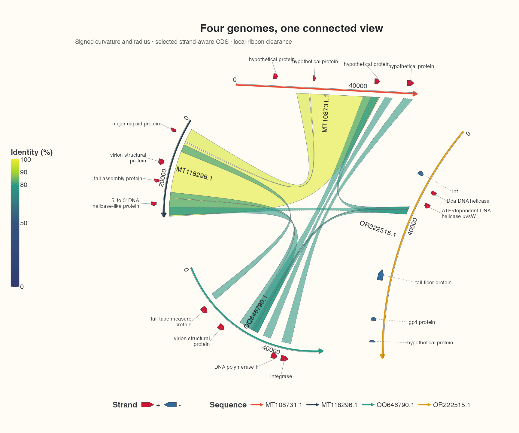
The original ggchord view, refined with signed curvature, varying radii, optimized display direction, local ribbon clearance and individually labelled selected features from real records. Data, complete code and interpretation →

Collinear · Four rows, many layers

Four-genome collinearity: strand-separated features and routed cross-row links · Click to enlarge

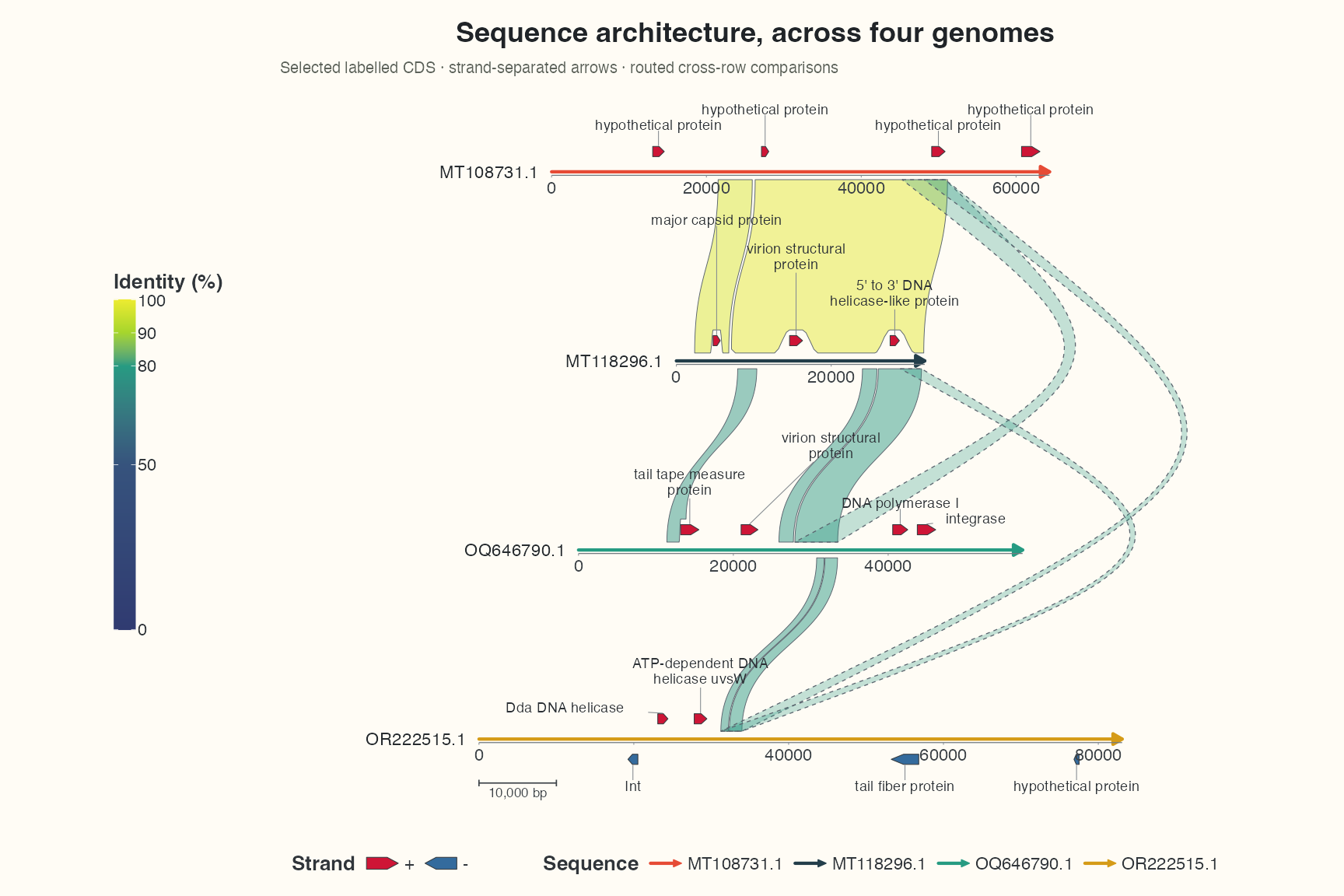
A linear expression of the chord grammar, reusing real sequences, observed alignments and the identity palette. Features separate by strand; long cross-row links route to the right. The tutorial demonstrates coordinate-only conversion and explains current circular-only parameter limits. Complete workflow and the meaning of each layer →

Plasmid · A richly annotated pETDuet-1

Dense pETDuet-1 map: features, reference primers and grouped restriction sites · Click to enlarge

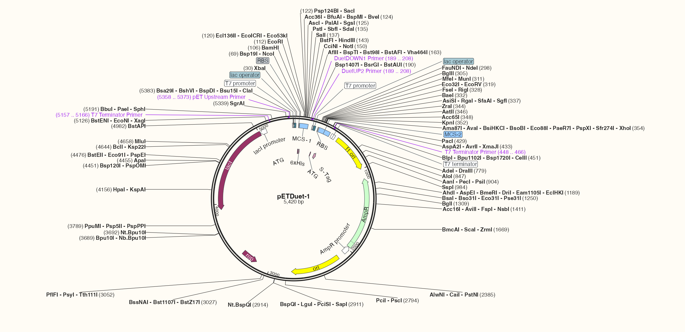
A double backbone, layered features, five reference primers and restriction-enzyme names grouped by shared cut position. The input includes 58 cut positions and 20 features; labels are laid out for the actual export size. From a first circular view to complete plasmid annotation →

Continue from where you are

• Install and draw a first plot
• Import your own data
• Adjust colours, legends and themes
• Browse all workflows and capabilities
• Look up functions, arguments and results

Examples prefer dplyr, purrr, tidyr and the native |> pipe, with ggplot2 layer composition. Updating older code? Read themigration guide.