Chapters and reference
Module II · Single-sequence circular maps · Section 4 of 12
2.3 Circular backbones and layout
On this page
Prepared annotations need only lengths and tables. DNA is used here to prepare the example annotation, not as a plotting requirement.
1 Input and provenance
Run independently in a fresh R session with optional dplyr. finish_features retains the first six recognition rows without changing intervals or strands. finish_labels appends actual coordinates to source names for label-fitting demonstrations; the original table remains separate.
R · Example code
library(ggchord)
library(dplyr)
finish_dna <- plasmid_example_pUC19
finish_seq <- finish_dna[c("accver", "length")]
finish_features <- head(find_common_features(finish_dna), 6)
finish_circle <- ggchord(finish_seq) + geom_seq() + coord_circular()
finish_labels <- finish_features |>
mutate(anno = paste0(anno, " [", start, "-", end, " bp]"))
finish_feature_base <- finish_circle + geom_feature(data = finish_labels)2 Backbone styles and double-line spacing
In single circular mode, seq_style = "auto" selects double. Single draws one backbone and double draws two. Keep the same sequence and 9 × 8 inch size, changing only style or double-line spacing. seq_backbone_gap defaults to 0.025; band width seq_backbone_width defaults to 0.035. Neither is stroke linewidth.
R · Example code
p_comparebonedouble <- ggchord(finish_seq) + geom_seq(seq_style = "double") + coord_circular()
view_ggchord(p_comparebonedouble, width = 9, height = 8, units = "in")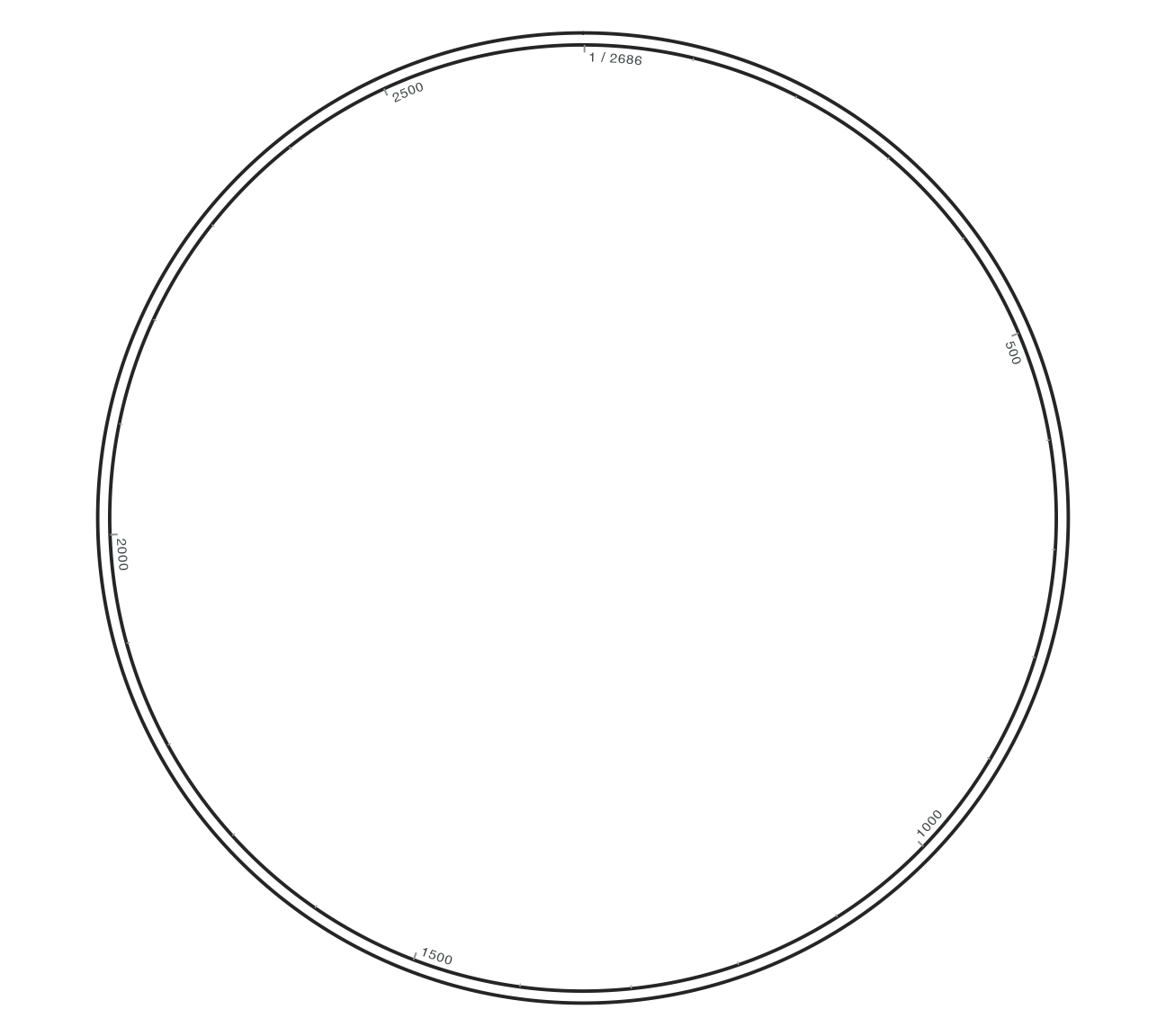
R · Example code
p_comparebonesingle <- ggchord(finish_seq) + geom_seq(seq_style = "single") + coord_circular()
view_ggchord(p_comparebonesingle, width = 9, height = 8, units = "in")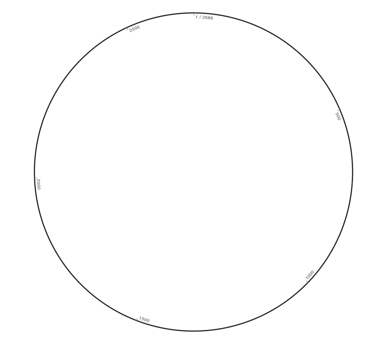
R · Example code
p_comparebonegap <- ggchord(finish_seq) + geom_seq(seq_style = "double", seq_backbone_gap = 0.05) + coord_circular()
view_ggchord(p_comparebonegap, width = 9, height = 8, units = "in")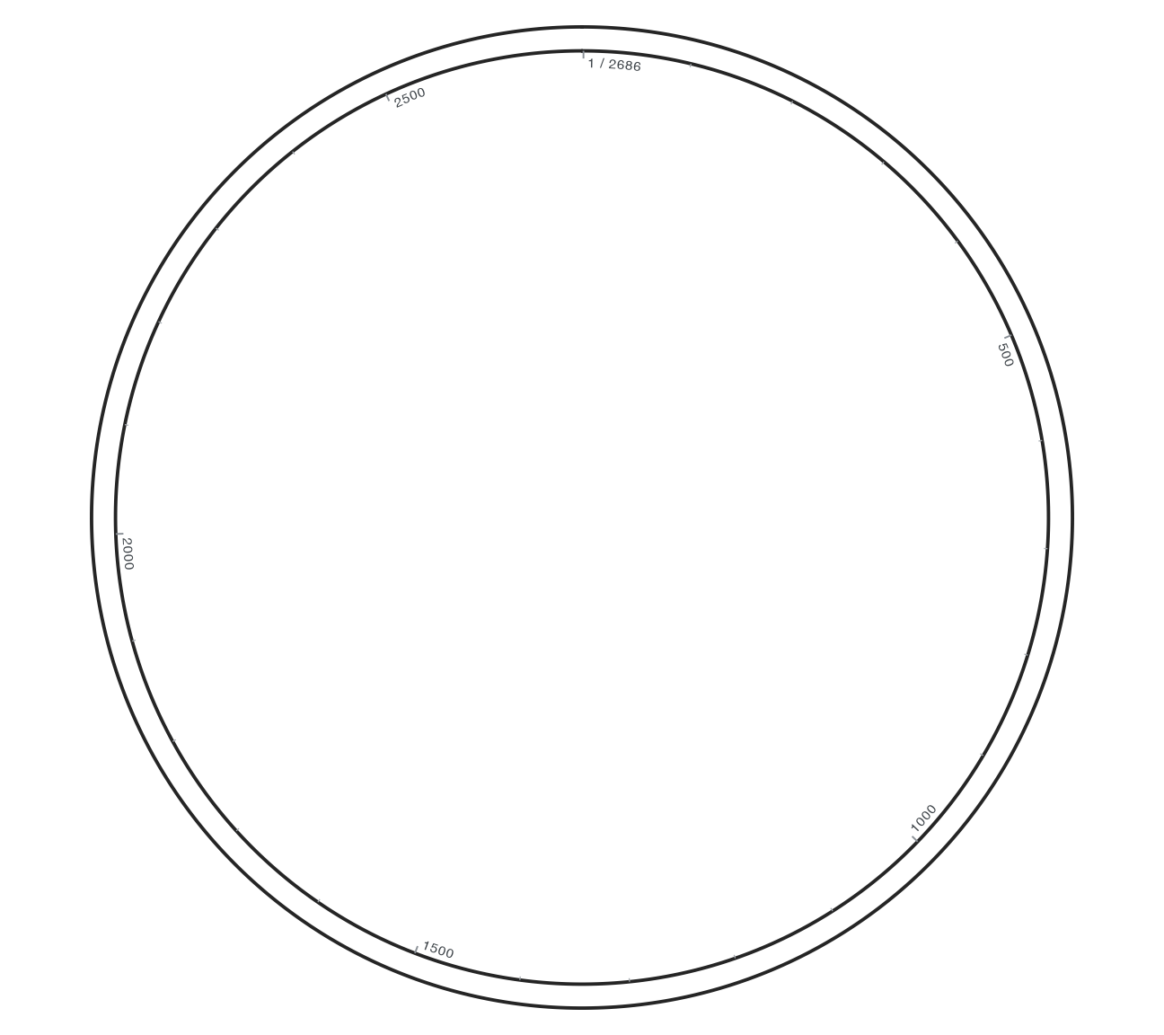
3 Band backbone
Band represents the complete backbone with a filled polygon. seq_backbone_width controls its width, default 0.035. This is actual band geometry; only seq_style changes from the double baseline.
R · Example code
p_compareboneband <- ggchord(finish_seq) + geom_seq(seq_style = "band") + coord_circular()
view_ggchord(p_compareboneband, width = 9, height = 8, units = "in")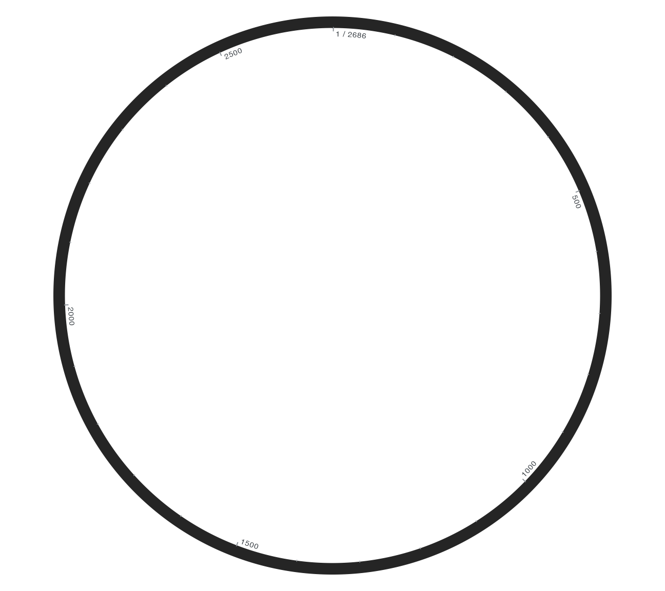
From the band baseline, double only band width while retaining other settings.
R · Example code
p_comparebandwidth <- ggchord(finish_seq) +
  geom_seq(seq_style = "band", seq_backbone_width = 0.07) + coord_circular()
view_ggchord(p_comparebandwidth, width = 9, height = 8, units = "in")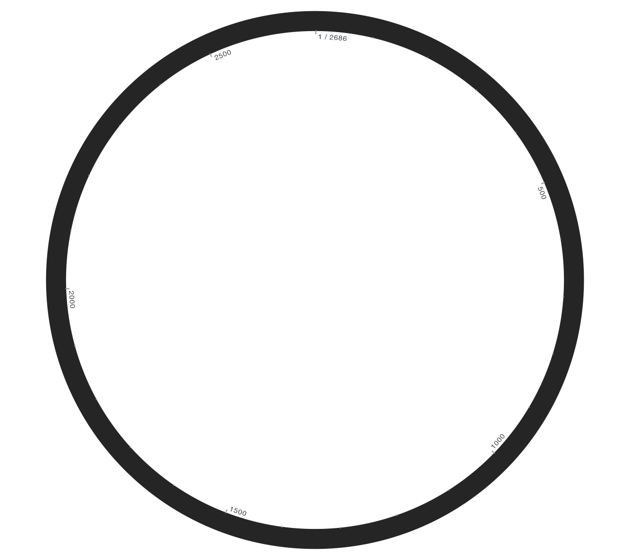
4 Circular direction, rotation, opening and fit
The zero origin is at 12 o’clock with clockwise coordinates. Positive rotation turns the complete plot counterclockwise. Relative to double above, each example changes only direction or gap. See the rotation contrast.
| Parameter | Default | Type and boundary |
|---|---|---|
rotation |
0 | Finite degrees; 90 places origin at 9 o’clock |
direction |
clockwise | clockwise/counterclockwise; not biological strand |
gap |
0 | Degrees in [0,360); does not remove bases |
fit |
labels | labels/geometry/manual; controls inclusion of labels in fitting |
ratio |
1 | Global aspect ratio, not a change in units |
clip |
off | Coordinate clipping can cut exterior text |
Automatic fitting may change overall scale and the readable subset of tick labels at fixed device size. Inspect text and leaders before fixing xlim/ylim; clipping is not loss of source data. Circular mode owns gap/direction and rejects geom_seq seq_gap/seq_orientation.
R · Example code
p_comparecirclecounter <- ggchord(finish_seq) + geom_seq(seq_style = "double") +
  coord_circular(direction = "counterclockwise")
view_ggchord(p_comparecirclecounter, width = 9, height = 8, units = "in")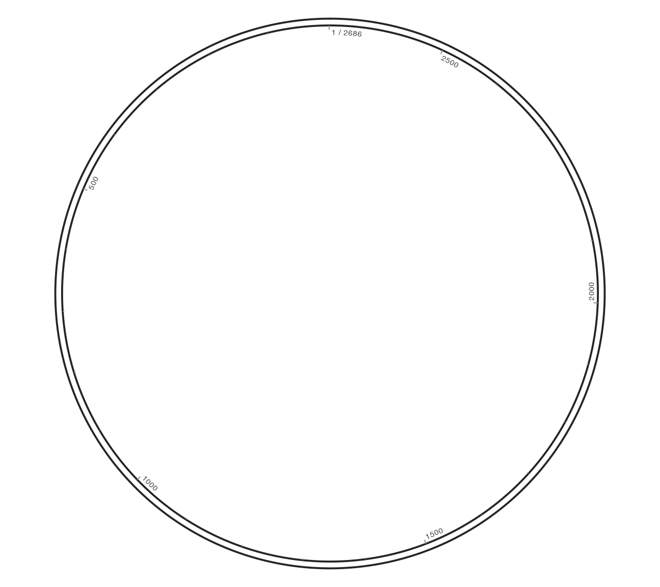
R · Example code
p_comparecirclegap <- ggchord(finish_seq) + geom_seq(seq_style = "double") +
  coord_circular(gap = 25)
view_ggchord(p_comparecirclegap, width = 9, height = 8, units = "in")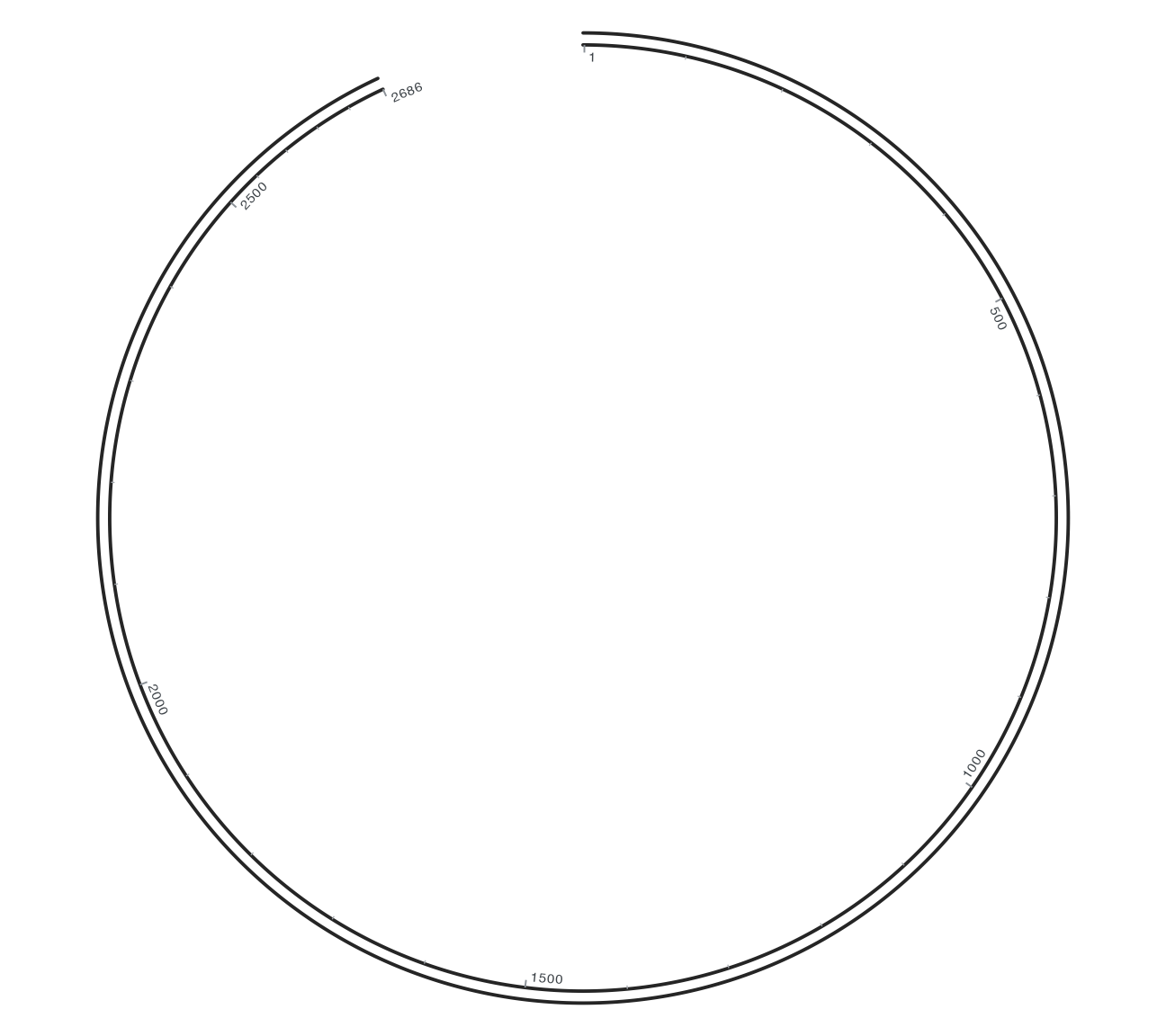
5 Style centre name and length separately
Centre text is separate from labels along the backbone. name = TRUE and length = TRUE are separated by a newline by default; name also accepts a display string. Empty name_style/length_style lists accept fixed colour, size, family, fontface and lineheight. First hide only length. Then return to baseline and change only name_style size, retaining the length text style.
R · Example code
p_comparecenter <- finish_circle + geom_seq_center_label()
view_ggchord(p_comparecenter, width = 9, height = 8, units = "in")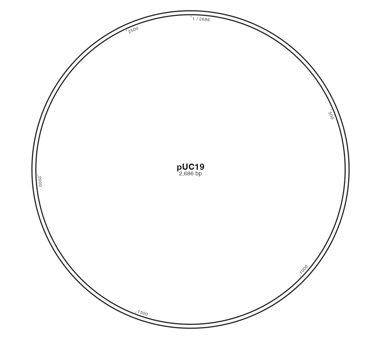
R · Example code
p_comparecenternolength <- finish_circle + geom_seq_center_label(length = FALSE)
view_ggchord(p_comparecenternolength, width = 9, height = 8, units = "in")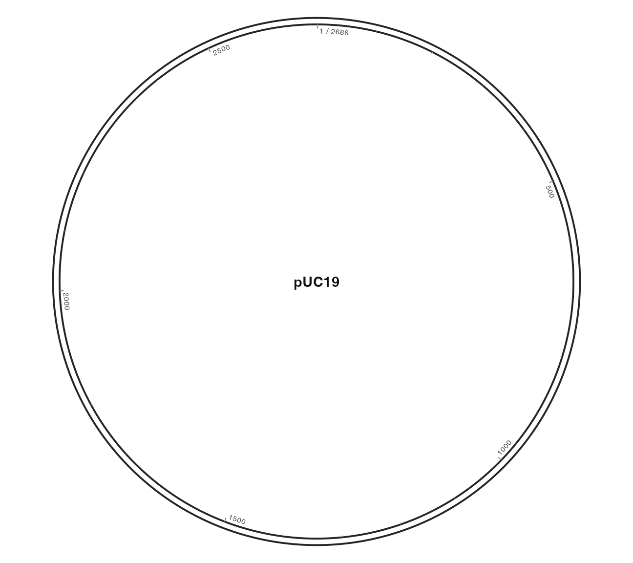
R · Example code
p_comparecenterstyle <- finish_circle +
  geom_seq_center_label(name_style = list(size = 6))
view_ggchord(p_comparecenterstyle, width = 9, height = 8, units = "in")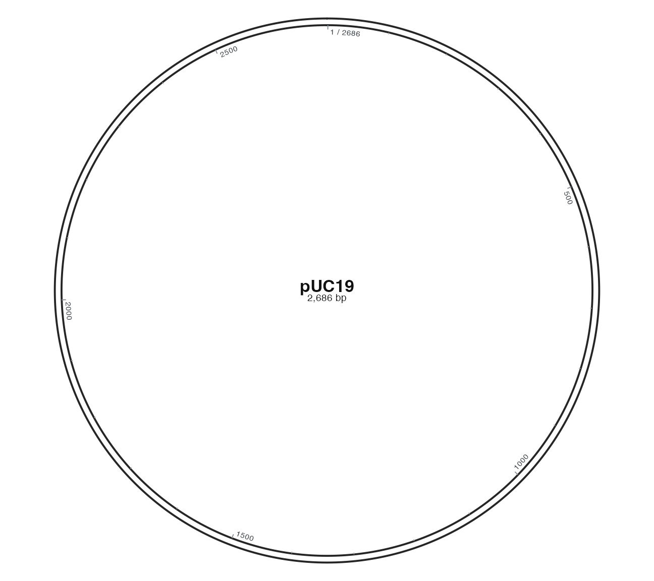
6 Switch to a single backbone
Data preparation and settings (expand)
R · Example code
plasmid <- plasmid_example_pUC19
p_first_circle <- ggchord(seq_data = plasmid) +
  geom_seq() +
  geom_seq_center_label() +
  coord_circular()
R · Example code
features <- find_common_features(plasmid)
origins <- subset(features, type == "rep_origin")
p_first_features <- p_first_circle +
  geom_feature_plasmid(data = origins)
R · Example code
p_circle_single <- ggchord(seq_data = plasmid) +
  geom_seq(seq_style = "single") +
  geom_seq_center_label() +
  coord_circular()
view_ggchord(p_circle_single, width = 6, height = 6, units = "in")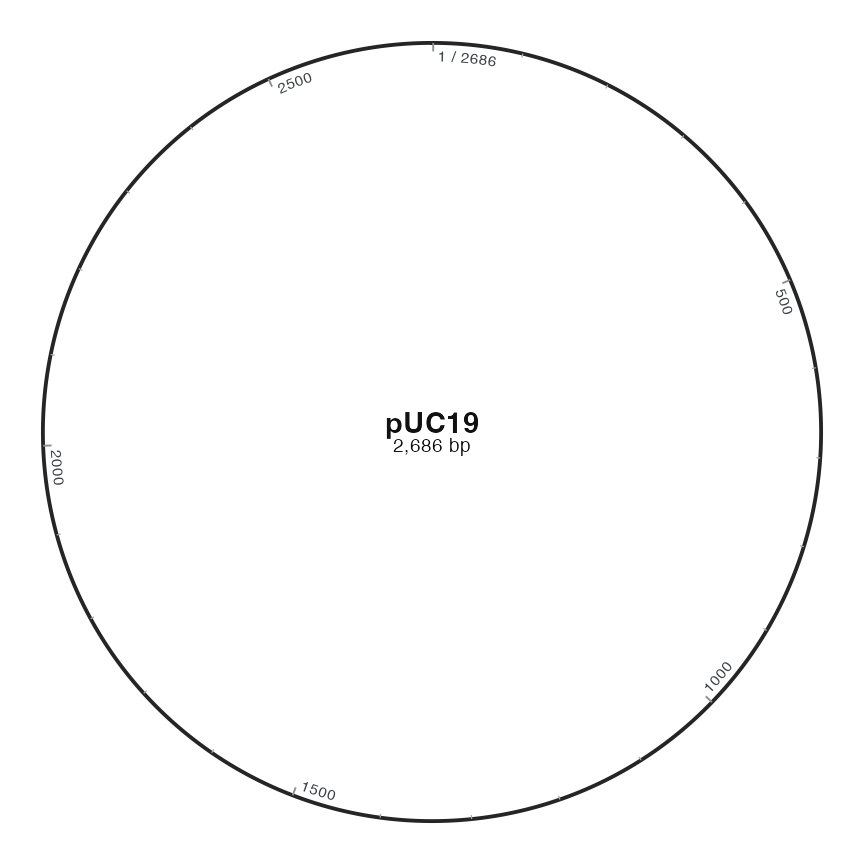
seq_style = "single" replaces the double backbone with one line. The centre label and bp ticks remain visible.
7 Rotate the map
R · Example code
features <- find_common_features(plasmid)
origins <- subset(features, type == "rep_origin")
p_first_features <- p_first_circle +
  geom_feature_plasmid(data = origins)

p_circle_rotated <- p_first_features + coord_circular(rotation = 90)
view_ggchord(p_circle_rotated, width = 6, height = 6, units = "in")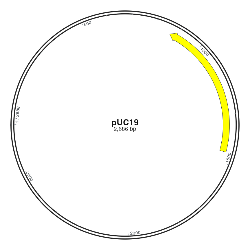
The default rotation = 0 places the sequence origin at 12 o’clock, with coordinates increasing clockwise. Here rotation = 90 moves it to 9 o’clock, rotating the ticks and replication origin together. The annotation still covers the same source bp interval. Next, prepare your own sequence and annotations.