Chapters and reference
Module II · Single-sequence circular maps · Section 2 of 12
2.1 Circular backbone and annotations
Download R scriptIncludes preparation and every page step. File examples need the input bundle; preview and save calls are retained.
1 Length and a prepared annotation
Only lengths and prepared tables are needed. The ori row is the verified pUC19 annotation 867–1455, matching the original inspectorigin output; no DNA recognition is run. Dependencies: ggchord and dplyr.
R · Example code
library(dplyr)
circle_seqs <- plasmid_example_pUC19 |> select(accver, length)
circle_origins <- tibble(
  accver = "pUC19", start = 867, end = 1455,
  strand = "-", type = "rep_origin", anno = "ori"
)
p_coursecircle <- ggchord(circle_seqs) +
  geom_seq() + geom_seq_center_label() + coord_circular()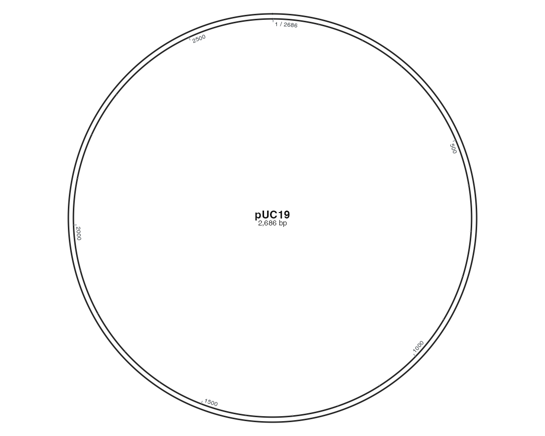
2 Add the feature and its label
R · Example code
p_coursecirclefeature <- p_coursecircle +
  geom_feature_plasmid(data = circle_origins) +
  geom_feature_label(data = circle_origins,
    label_side = "inside", label_radial_offset = 0.12, size = 4)
view_ggchord(p_coursecirclefeature, width = 10, height = 8, units = "in")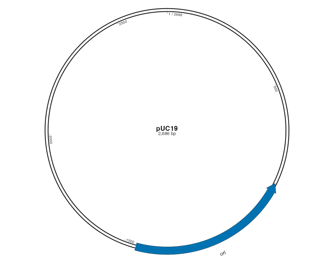
Locate both ori endpoints on the ticks and trace the label to anno. A circular display is not evidence of molecular topology.
3 Preview and save
Remove the label layer and rerun; backbone and source interval stay unchanged. Replace the row with your own known annotation.
R · Example code
circular_width <- 10
circular_height <- 8
view_ggchord(p_coursecirclefeature,
  width = circular_width, height = circular_height, units = "in")
ggsave("circular-first.png", p_coursecirclefeature,
  width = circular_width, height = circular_height, units = "in", dpi = 144)