章节与参考
模块二 · 单序列圆图 · 第 4 节,共 12 节
2.3 圆图骨架与布局
已有注释只需长度与表格;本页为了获得真实示例注释才读取 DNA。
1 本页输入与来源
本页在新 R 会话独立运行,需可选依赖 dplyr。finish_features 保留识别结果的前六行,不改变区间与链。为比较标签适配,finish_labels 的显示文字在原始名称后附上真实坐标,原始表仍单独保存。
R · 示例代码
library(ggchord)
library(dplyr)
finish_dna <- plasmid_example_pUC19
finish_seq <- finish_dna[c("accver", "length")]
finish_features <- head(find_common_features(finish_dna), 6)
finish_circle <- ggchord(finish_seq) + geom_seq() + coord_circular()
finish_labels <- finish_features |>
mutate(anno = paste0(anno, " [", start, "-", end, " bp]"))
finish_feature_base <- finish_circle + geom_feature(data = finish_labels)2 骨架样式与双线间距
seq_style = "auto" 在单圆图中选择双线;single 是一条骨架,double 是双线。下面保持 9 × 8 英寸与同一序列,每次只改变样式或双线间距。双线间距 seq_backbone_gap 默认 0.025,band 的宽度参数 seq_backbone_width 默认 0.035,二者不是线条的 linewidth。
R · 示例代码
p_comparebonedouble <- ggchord(finish_seq) + geom_seq(seq_style = "double") + coord_circular()
view_ggchord(p_comparebonedouble, width = 9, height = 8, units = "in")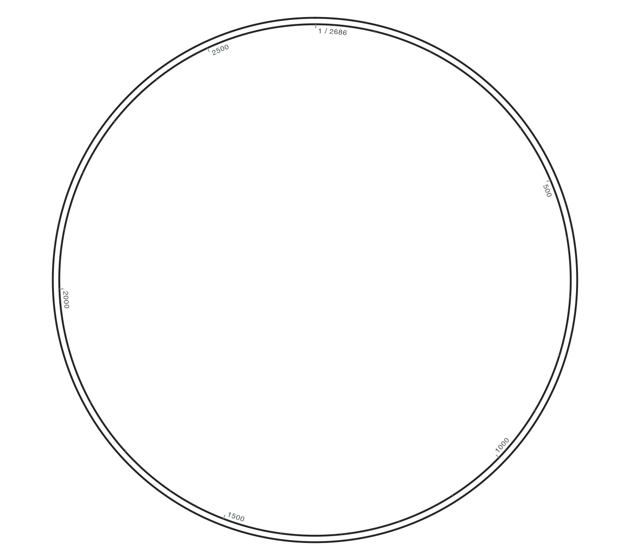
R · 示例代码
p_comparebonesingle <- ggchord(finish_seq) + geom_seq(seq_style = "single") + coord_circular()
view_ggchord(p_comparebonesingle, width = 9, height = 8, units = "in")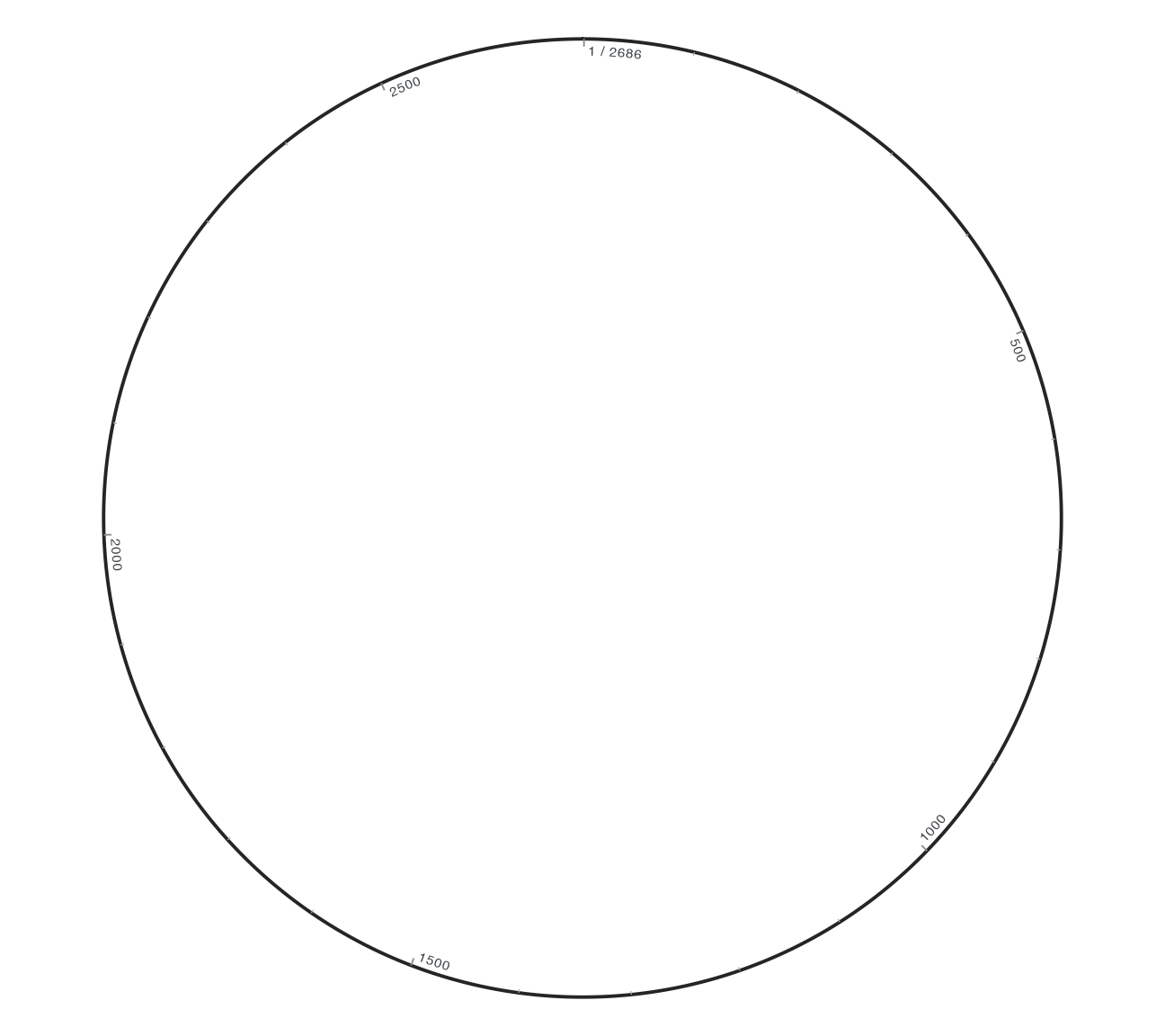
R · 示例代码
p_comparebonegap <- ggchord(finish_seq) + geom_seq(seq_style = "double", seq_backbone_gap = 0.05) + coord_circular()
view_ggchord(p_comparebonegap, width = 9, height = 8, units = "in")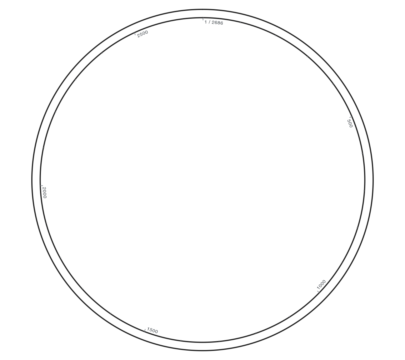
3 band 色带骨架
band 用填充多边形表示整条骨架,宽度由 seq_backbone_width 控制,默认 0.035。以下使用真实 band 骨架,与双线图相比只改变 seq_style。
R · 示例代码
p_compareboneband <- ggchord(finish_seq) + geom_seq(seq_style = "band") + coord_circular()
view_ggchord(p_compareboneband, width = 9, height = 8, units = "in")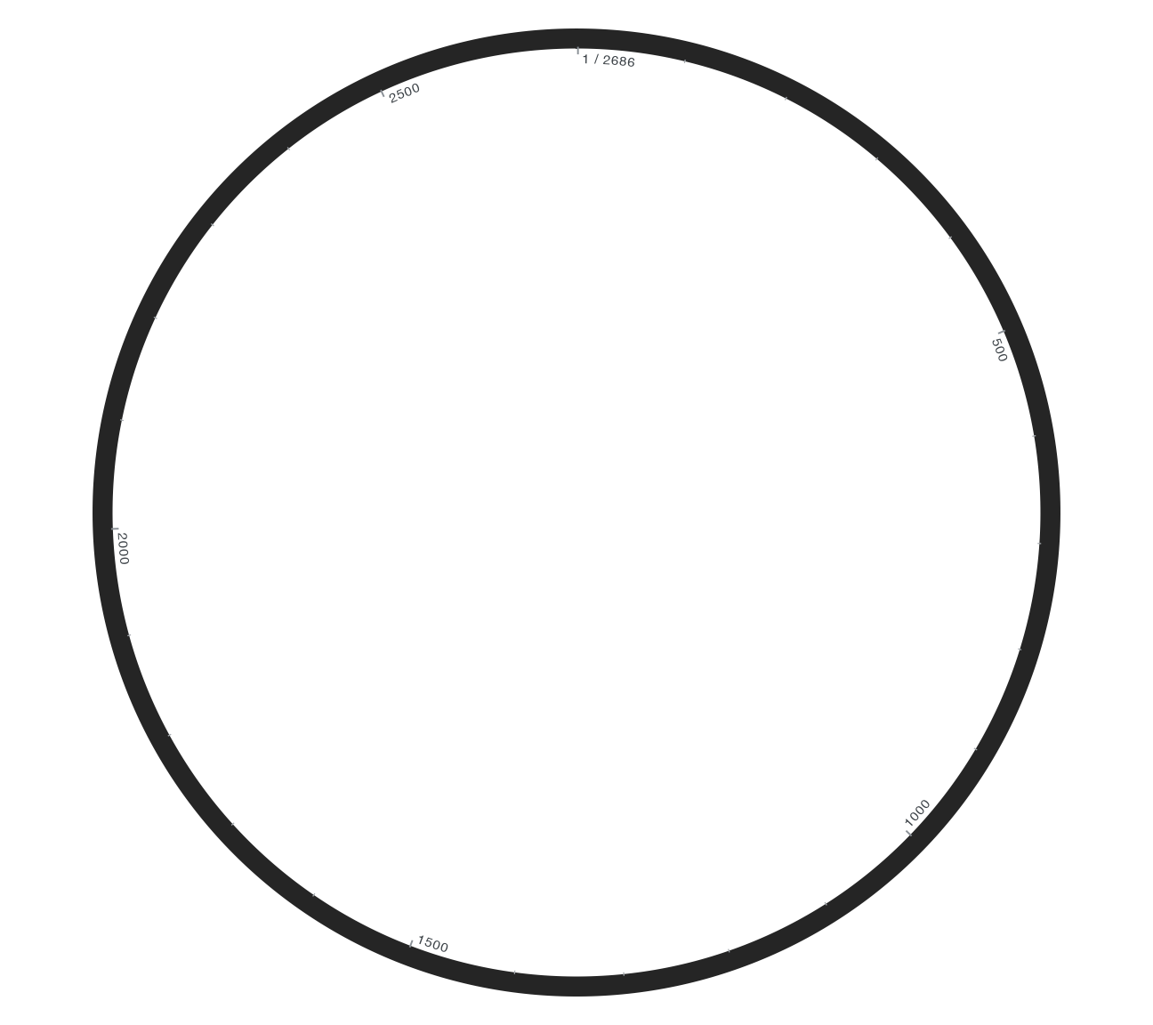
同一 band 基线,只把宽度加倍;其他设置不变。
R · 示例代码
p_comparebandwidth <- ggchord(finish_seq) +
  geom_seq(seq_style = "band", seq_backbone_width = 0.07) + coord_circular()
view_ggchord(p_comparebandwidth, width = 9, height = 8, units = "in")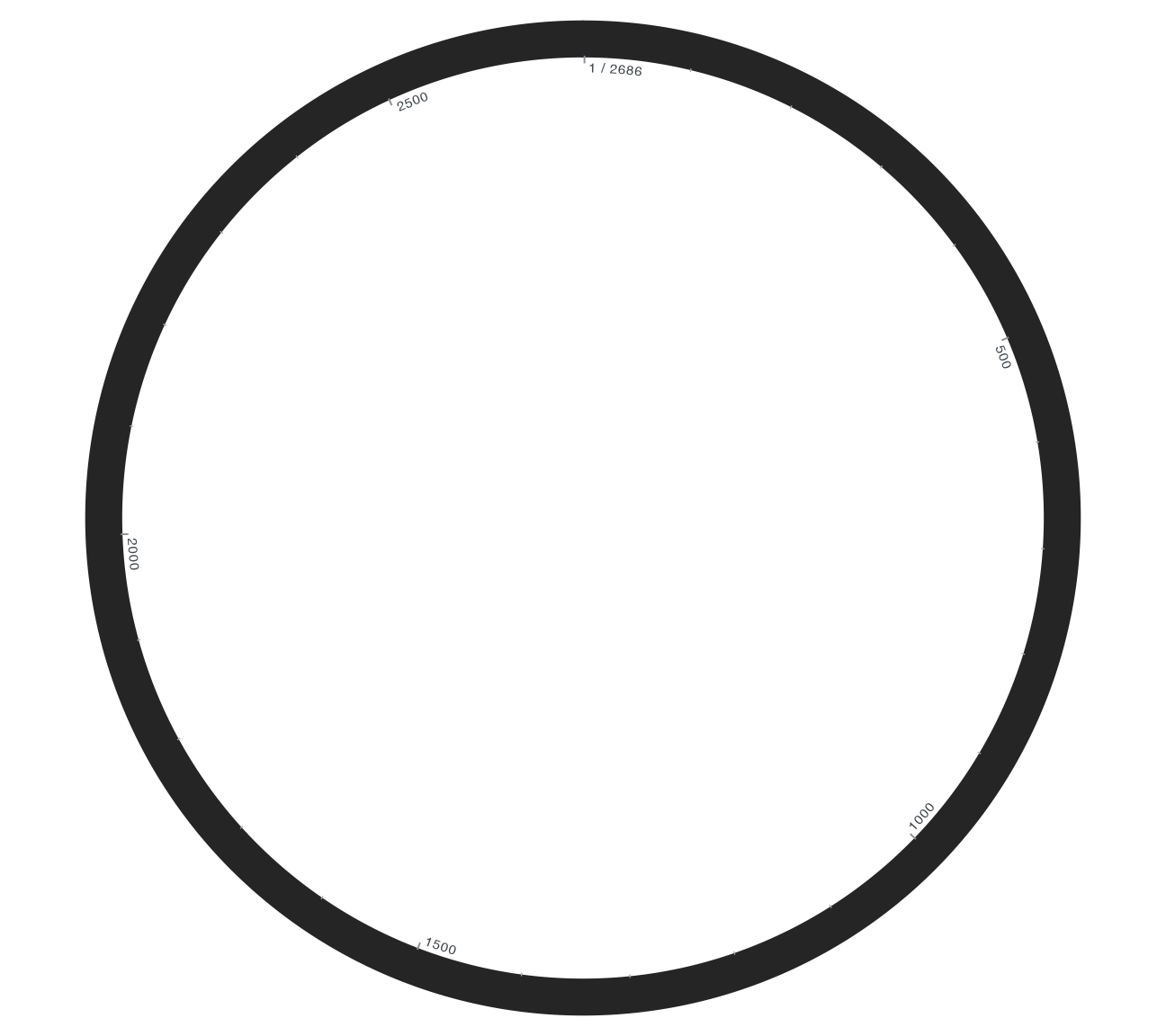
4 圆图坐标、旋转、开口与适配
零旋转的原点在 12 点钟,默认顺时针增加;正 rotation 逆时针转动整图。与上面 double 基线相比,下面分别只改变 direction 或 gap。rotation 对照见圆图旋转。
| 参数 | 默认 | 类型与边界 |
|---|---|---|
rotation |
0 | 有限数值,角度;90 是九点钟 |
direction |
clockwise | clockwise/counterclockwise;不是生物学链 |
gap |
0 | [0,360) 度;不从序列中删除碱基 |
fit |
labels | labels/geometry/manual;是否将标签纳入适配 |
ratio |
1 | 全局纵横比,不改变长度单位 |
clip |
off | 裁剪由坐标控制;打开裁剪可能截掉外侧文字 |
固定尺寸下,自动适配会改变整体缩放和可读刻度标签的子集。手动限制 xlim/ylim 时先检查文字和引线,不把裁剪误认为数据丢失。圆图用 gap/direction,不能传入 geom_seq 的 seq_gap/seq_orientation。
R · 示例代码
p_comparecirclecounter <- ggchord(finish_seq) + geom_seq(seq_style = "double") +
  coord_circular(direction = "counterclockwise")
view_ggchord(p_comparecirclecounter, width = 9, height = 8, units = "in")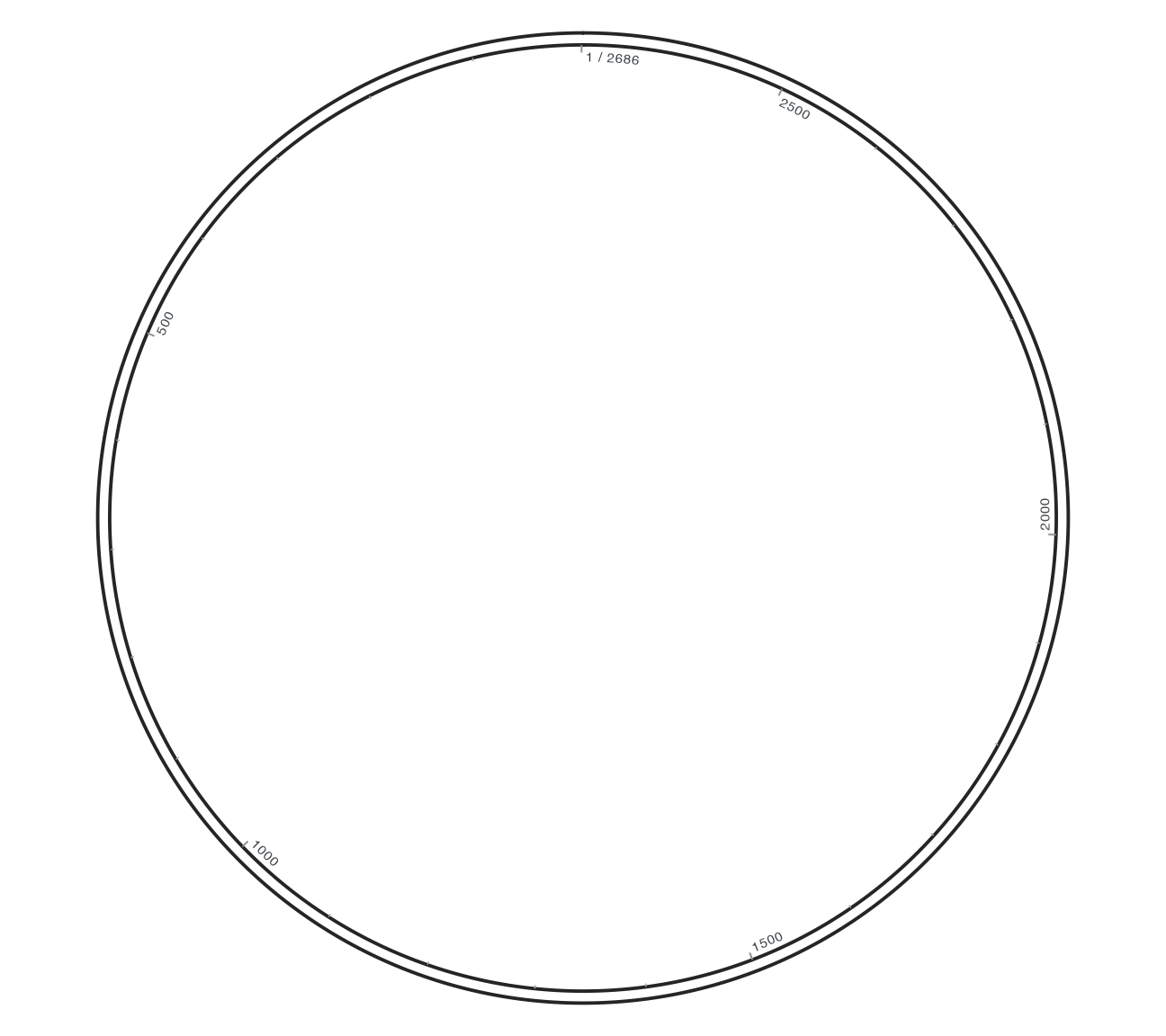
R · 示例代码
p_comparecirclegap <- ggchord(finish_seq) + geom_seq(seq_style = "double") +
  coord_circular(gap = 25)
view_ggchord(p_comparecirclegap, width = 9, height = 8, units = "in")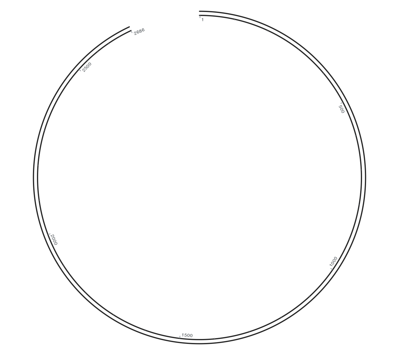
5 分别设置中心名称和长度
中心文字与沿骨架的序列标签是不同图层。name = TRUE、length = TRUE,默认用换行符 separator 分隔;name 也可提供显示字符串。name_style/length_style 默认空列表,接受固定 colour、size、family、fontface、lineheight。下面先只隐藏 length,再回到基线只改变 name_style 的 size,长度字号不会跟着改变。
R · 示例代码
p_comparecenter <- finish_circle + geom_seq_center_label()
view_ggchord(p_comparecenter, width = 9, height = 8, units = "in")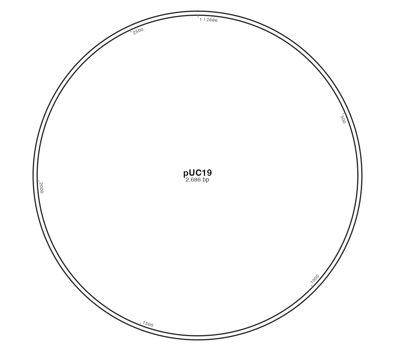
R · 示例代码
p_comparecenternolength <- finish_circle + geom_seq_center_label(length = FALSE)
view_ggchord(p_comparecenternolength, width = 9, height = 8, units = "in")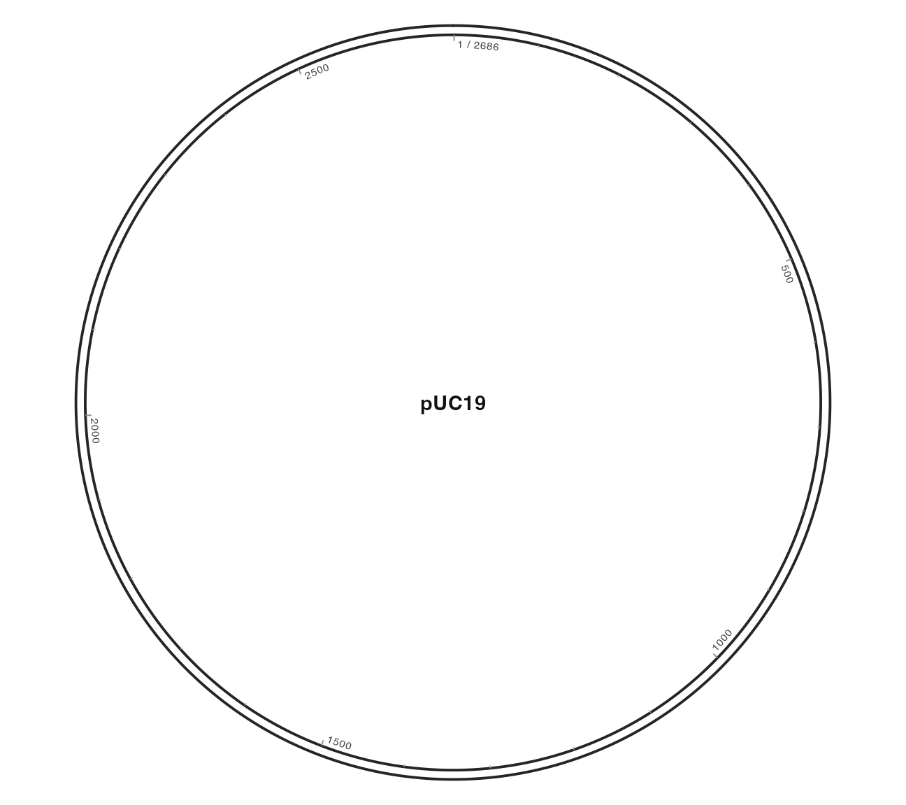
R · 示例代码
p_comparecenterstyle <- finish_circle +
  geom_seq_center_label(name_style = list(size = 6))
view_ggchord(p_comparecenterstyle, width = 9, height = 8, units = "in")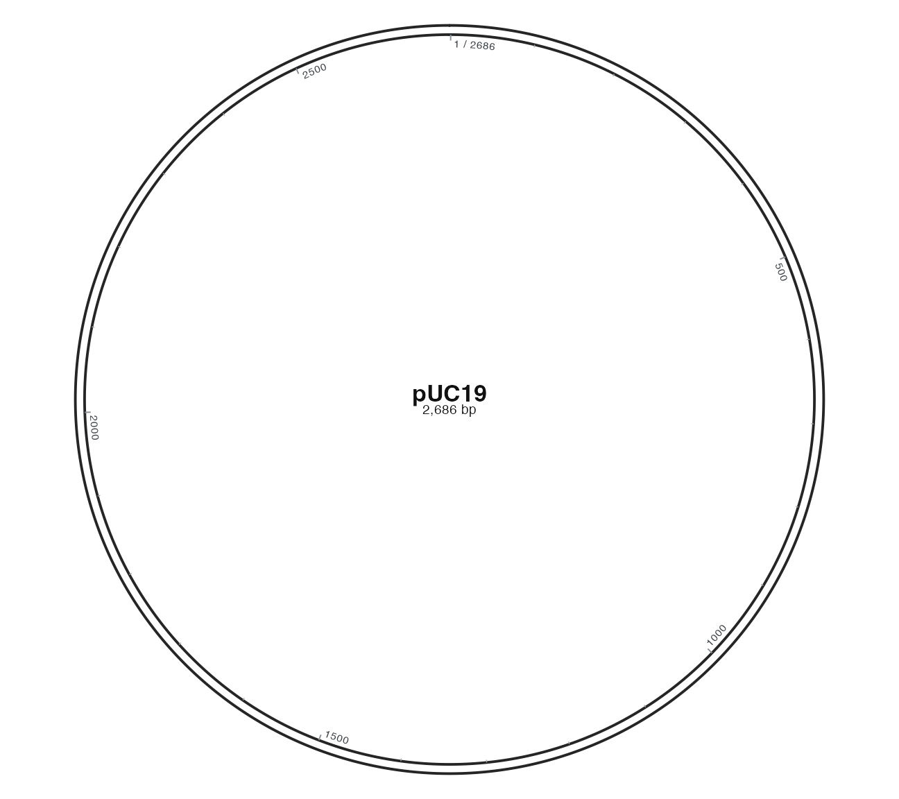
6 切换为单线骨架
准备数据与配置(展开)
R · 示例代码
plasmid <- plasmid_example_pUC19
p_first_circle <- ggchord(seq_data = plasmid) +
  geom_seq() +
  geom_seq_center_label() +
  coord_circular()
R · 示例代码
features <- find_common_features(plasmid)
origins <- subset(features, type == "rep_origin")
p_first_features <- p_first_circle +
  geom_feature_plasmid(data = origins)
R · 示例代码
p_circle_single <- ggchord(seq_data = plasmid) +
  geom_seq(seq_style = "single") +
  geom_seq_center_label() +
  coord_circular()
view_ggchord(p_circle_single, width = 6, height = 6, units = "in")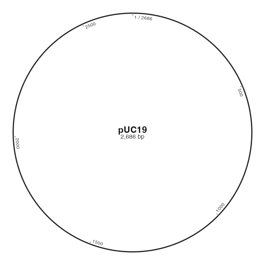
seq_style = "single" 把双线改为单线。中心名称和 bp 刻度仍可用于定位。
7 转动圆图
R · 示例代码
features <- find_common_features(plasmid)
origins <- subset(features, type == "rep_origin")
p_first_features <- p_first_circle +
  geom_feature_plasmid(data = origins)

p_circle_rotated <- p_first_features + coord_circular(rotation = 90)
view_ggchord(p_circle_rotated, width = 6, height = 6, units = "in")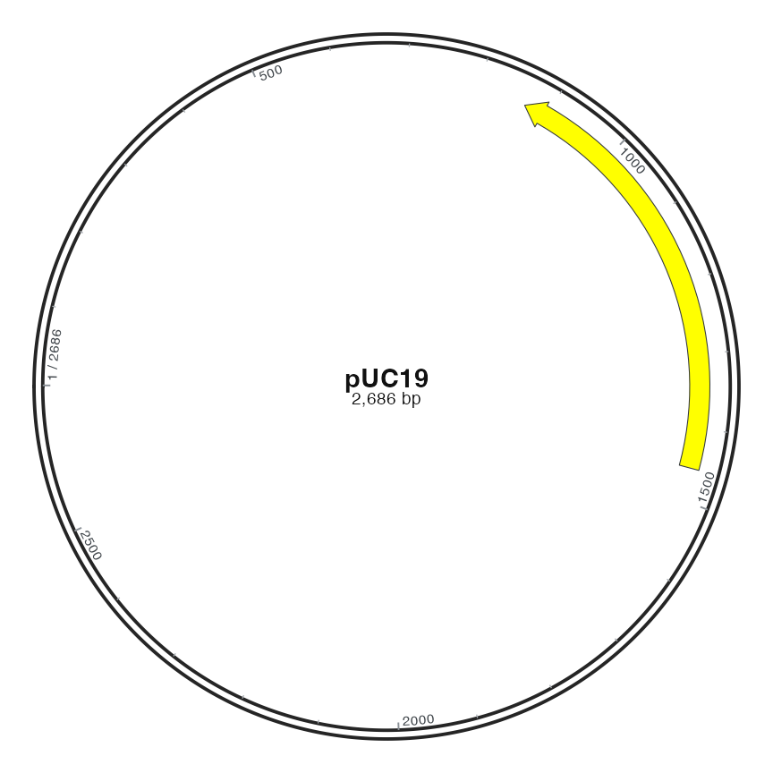
默认 rotation = 0 把序列起点放在 12 点钟,坐标顺时针增加。这里设置 rotation = 90,起点移到 9 点钟;圆周刻度和复制起点一起旋转。原始注释区间仍是同一段 bp。下一节整理自己的序列和注释。