0.16.6 documentation

Site guide · find your task

Setup and learning paths

HomeInstall and prepare the environmentChoose your learning module

Module I · Chord

1.1 Tables and field meanings1.2 Produce and import comparisons1.3 Build the layers step by step1.4 Direction, curvature and clearance1.5 Filter and summarize links1.6 Full source-file workflow1.7 Complete chord showcase

Module II · Collinear

2.1 Reuse chord input tables2.2 Switch coordinates and add layers2.3 Routes, clearance and the ruler2.4 Compare CDS neighbourhoods2.5 Focus, anchors and segments2.6 Complete collinear showcase

Module III · Plasmid

3.1 DNA, annotations and 13 references3.2 From a circle to annotation layers3.3 Features, primers and restriction3.4 Thirteen plasmid references3.5 Complete plasmid cases

Consult as needed · Data and layers

Prepare tables and coordinatesImport and convert dataImport nucleotide and protein alignmentsProject protein intervals to genomic coordinatesFeatures, stacking and genomic decorationLabels and local placementQuantitative tracksMappings, scales, guides and themesSet values by sequence and strandCommon adjustments and grammarExport, preview and diagnostics

Learning map and reference

Articles and complete workflowsFunction referenceReproducible galleryFrequently asked questionsMigrate to the candidate APITerminology and design sourcesDevelopment status and changes

3.2 From a circle to annotation layers

On this page

• Prepare this page
• Step 1: double backbone and centre name
• Step 2: feature shapes
• Step 3: fitted feature labels
• Step 4: primers and selected restriction sites

Focus on the visual information added at each step. Preparation computes inputs; independent layers still control drawing.

Prepare this page

Preparation code — run once on this page

Code

library(ggchord)
feature_palette <- c(
  CDS = "#993366", promoter = "#31849B", rep_origin = "#F1E51D",
  primer_bind = "#A020F0", misc_feature = "#A6ACB3", protein_bind = "#31849B"
)

library(ggchord)
doc_background <- "#FFFCF5"
identity_palette <- c("#303B71", "#36537D", "#269B82", "#A5D52C", "#ECEB31")
identity_values <- c(0, 0.5, 0.8, 0.9, 1)
identity_breaks <- c(0, 50, 80, 90, 100)
doc_legend_theme <- theme(
  legend.title = element_text(size = 13, face = "bold"),
  legend.text = element_text(size = 11),
  legend.key.width = unit(9, "mm"), legend.key.height = unit(5, "mm"),
  legend.spacing.x = unit(9, "mm"), legend.spacing.y = unit(7, "mm"),
  legend.margin = margin(l = 4, r = 4, unit = "mm")
)
sequence_guide <- guide_ggchord_legend(nrow = 1, theme = doc_legend_theme)
strand_guide <- guide_ggchord_legend(
  nrow = 1, override.aes = list(strand = c("+", "-")), theme = doc_legend_theme
)
identity_guide <- guide_ggchord_colourbar(
  position = "left", direction = "vertical",
  theme = theme(
    legend.key.height = unit(75, "mm"), legend.key.width = unit(5, "mm"),
    legend.title = element_text(size = 13, face = "bold"),
    legend.text = element_text(size = 11), legend.margin = margin(r = 7, unit = "mm")
  )
)
doc_theme <- theme_ggchord_publication(
  axis.text = element_text(size = 11),
  axis.text.check.overlap = TRUE
) +
  theme(
    legend.position = "bottom",
    legend.title = element_text(size = 13, face = "bold"),
    legend.text = element_text(size = 11),
    legend.key.width = unit(9, "mm"), legend.key.height = unit(5, "mm"),
    legend.spacing.x = unit(9, "mm"), legend.spacing.y = unit(7, "mm"),
    legend.box.spacing = unit(6, "mm"),
    plot.background = element_rect(fill = doc_background, colour = NA),
    panel.background = element_blank(),
    plot.title = element_text(face = "bold", size = 18),
    plot.subtitle = element_text(size = 10, colour = "#5C625A"),
    plot.margin = margin(14, 18, 14, 18)
  )
doc_axis <- function(coordinates = "relative") {
  scale_seq_position_continuous(
    coordinates = coordinates, n.breaks = 3, minor_breaks = NULL,
    labels = function(x) format(x, scientific = FALSE, big.mark = ",", trim = TRUE)
  )
}

library(dplyr)
data(plasmid_example_pUC19)
plasmid_seq <- plasmid_example_pUC19 |>
  select(accver, length)
plasmid_feature_source <- find_common_features(plasmid_example_pUC19)
# Dedicated primer layers already show bindings; avoid duplicate primer annotations.
plasmid_features <- plasmid_feature_source |>
  filter(type != "primer_bind") |>
  select(accver, start, end, strand, type, anno)
plasmid_primers <- find_primer_bindings(plasmid_example_pUC19, set = "universal")
plasmid_sites <- find_restriction_sites(plasmid_example_pUC19)
display_sites <- filter_restriction_sites(plasmid_sites, enzymes = c("EcoRI", "BamHI", "HindIII"))
primer_names <- primer_catalog(set = "universal")

Code

plasmid_position <- position_feature_stack(spacing = 0.085, base_position = position_plasmid())
p_plasmid_backbone <- ggchord(seq_data = plasmid_seq) +
  geom_seq(seq_style = "double", colour = "#252525") +
  geom_seq_center_label() +
  coord_circular(rotation = 90) +
  theme_ggchord_plasmid() +
  theme(
    panel.background = element_blank(),
    plot.background = element_rect(fill = doc_background, colour = NA)
  )
p_plasmid_features <- p_plasmid_backbone +
  geom_feature_plasmid(data = plasmid_features, position = plasmid_position)
p_plasmid_text <- p_plasmid_features +
  geom_feature_label_repel(
    data = plasmid_features, position = plasmid_position,
    external = TRUE, label_fit = "shrink", label_min_size = 2.5
  )
p_plasmid_text

Step 1: double backbone and centre name

pUC19 step1: double backbone · Click to enlarge

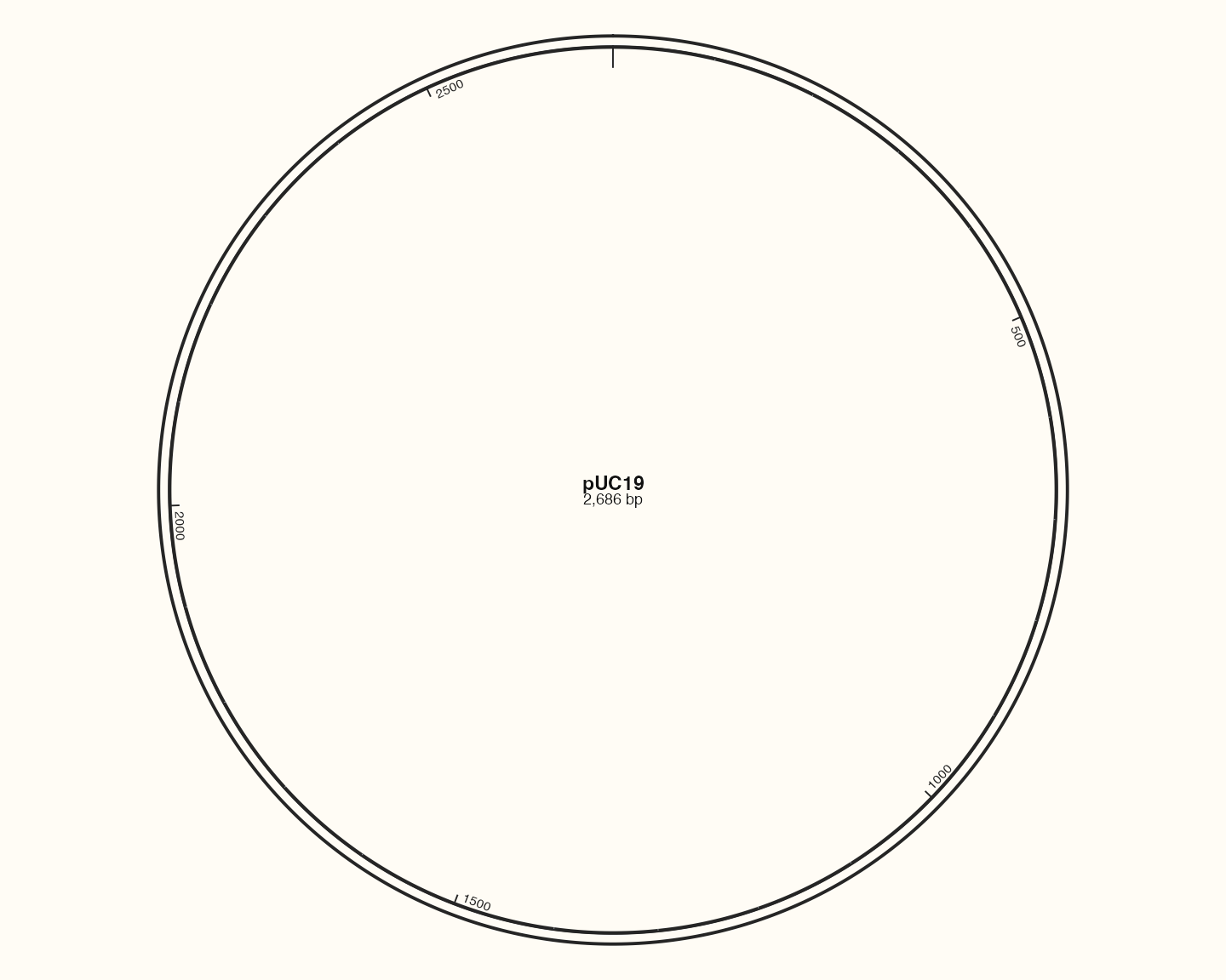
Check name and full length first. coord_circular() accepts one sequence; the geom owns the double-line style.

Step 2: feature shapes

pUC19 step2: features · Click to enlarge

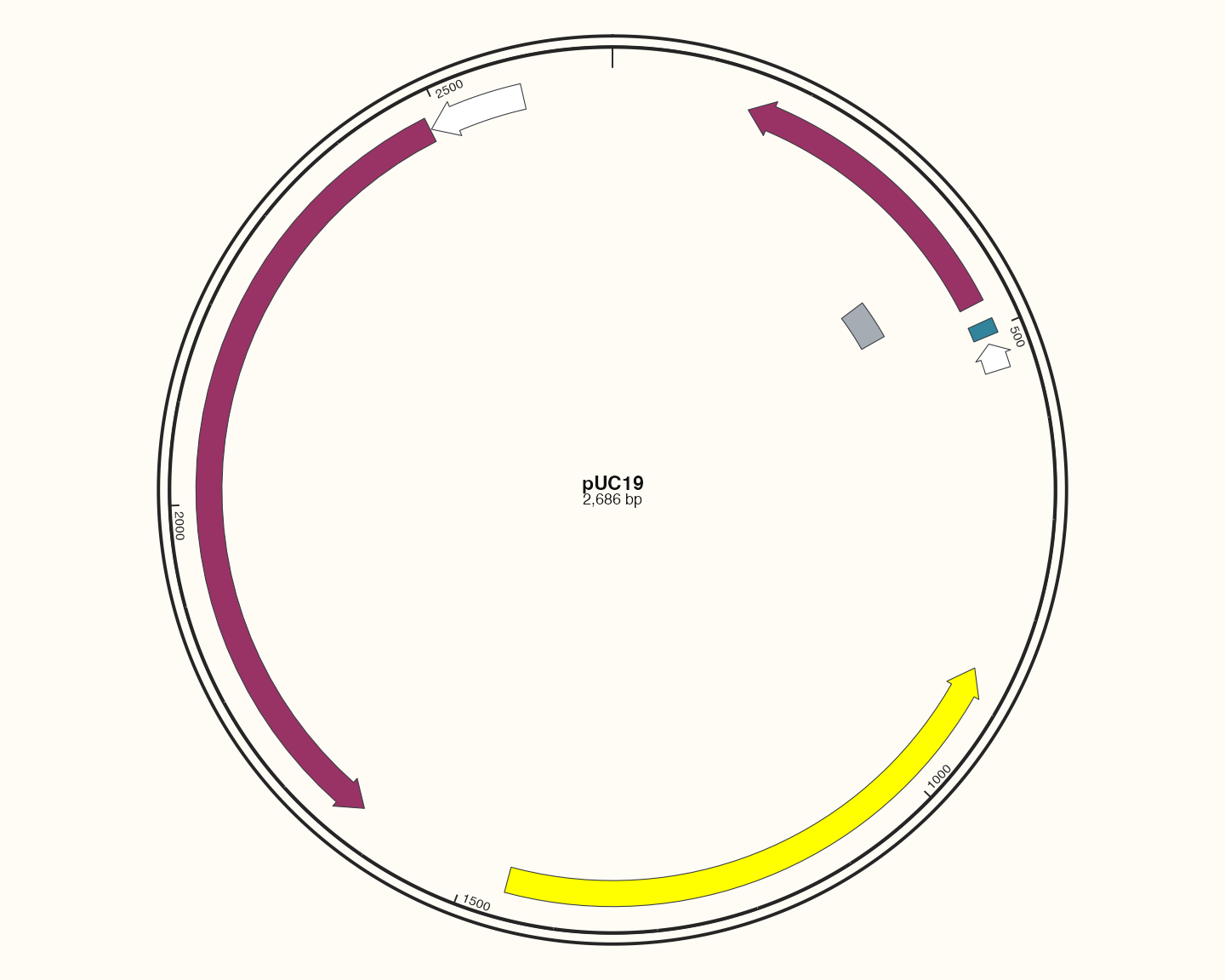
position_feature_stack() separates overlaps; geom_feature_plasmid() selects shapes and colours by real category. Compact short-feature shapes do not imply missing data.

Step 3: fitted feature labels

pUC19 step3: labels · Click to enlarge

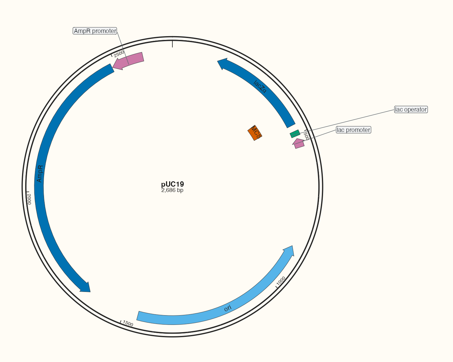
Geometry and labels share a Position. Allow shrinking only above an explicit minimum and external placement when necessary; recheck after changing dimensions.

Step 4: primers and selected restriction sites

Code

plasmid_position <- position_feature_stack(spacing = .10, base_position = position_plasmid())
p_plasmid <- ggchord(seq_data = plasmid_seq) +
  geom_seq(seq_style = "double") +
  geom_feature_plasmid(aes(feature_fill = type), data = plasmid_features, position = plasmid_position) +
  geom_feature_label_repel(
    data = plasmid_features, position = plasmid_position,
    size = 4
  ) +
  geom_primer(data = plasmid_primers, colour = "#A020F0") +
  geom_primer_label_repel(data = plasmid_primers, colour = "#A020F0", max_overlaps = 0, size = 3) +
  geom_restriction_site(data = display_sites, colour = "#29364B", label_size = 3, leader = "radial") +
  geom_seq_center_label() +
  scale_feature_fill_manual(values = feature_palette) +
  scale_seq_position_continuous() +
  coord_circular(rotation = 90) +
  theme_ggchord_plasmid() +
  theme(
    legend.title = element_text(size = 13, face = "bold"),
    legend.text = element_text(size = 11),
    legend.spacing.x = unit(9, "mm"), legend.spacing.y = unit(7, "mm"),
    plot.background = element_rect(fill = doc_background, colour = NA),
    panel.background = element_blank()
  )
p_plasmid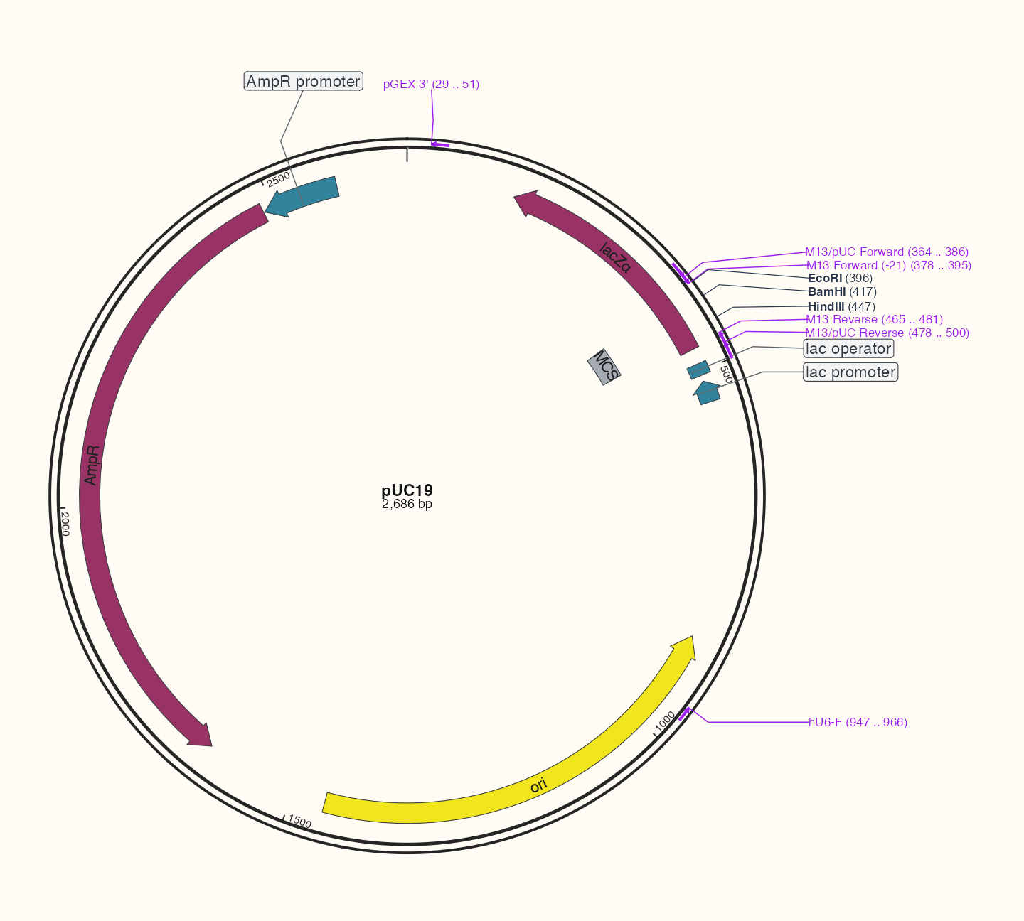

pUC19 features, exact primer hits and three selected restriction sites · Click to enlarge

Only three selected enzyme sites are displayed; the full search table remains available. See 3.3 for recognition provenance and assumptions. Compare annotation densities across 13 references, then finish the dense pETDuet-1 showcase.