Site guide · find your task
2.3 Routes, clearance and the ruler
On this page
Adjacent and cross-row links impose different reading costs. Separate their data and controls while preserving observed HSP endpoints. Control points change display paths only.
Prepare this page
Extract the input bundle first.Preparation code — run once on this page
Code
# Optional appearance choices; none of these columns or scales is required input.
library(ggchord)
seq_palette <- setNames(
  c("#E64B35", "#233E4A", "#269B82", "#D59B17"),
  c("MT108731.1", "MT118296.1", "OQ646790.1", "OR222515.1")
)
gene_palette <- c("+" = "#CE1536", "-" = "#346B9D", "." = "#8291A6")

library(ggchord)
doc_background <- "#FFFCF5"
identity_palette <- c("#303B71", "#36537D", "#269B82", "#A5D52C", "#ECEB31")
identity_values <- c(0, 0.5, 0.8, 0.9, 1)
identity_breaks <- c(0, 50, 80, 90, 100)
doc_legend_theme <- theme(
  legend.title = element_text(size = 13, face = "bold"),
  legend.text = element_text(size = 11),
  legend.key.width = unit(9, "mm"), legend.key.height = unit(5, "mm"),
  legend.spacing.x = unit(9, "mm"), legend.spacing.y = unit(7, "mm"),
  legend.margin = margin(l = 4, r = 4, unit = "mm")
)
sequence_guide <- guide_ggchord_legend(nrow = 1, theme = doc_legend_theme)
strand_guide <- guide_ggchord_legend(
  nrow = 1, override.aes = list(strand = c("+", "-")), theme = doc_legend_theme
)
identity_guide <- guide_ggchord_colourbar(
  position = "left", direction = "vertical",
  theme = theme(
    legend.key.height = unit(75, "mm"), legend.key.width = unit(5, "mm"),
    legend.title = element_text(size = 13, face = "bold"),
    legend.text = element_text(size = 11), legend.margin = margin(r = 7, unit = "mm")
  )
)
doc_theme <- theme_ggchord_publication(
  axis.text = element_text(size = 11),
  axis.text.check.overlap = TRUE
) +
  theme(
    legend.position = "bottom",
    legend.title = element_text(size = 13, face = "bold"),
    legend.text = element_text(size = 11),
    legend.key.width = unit(9, "mm"), legend.key.height = unit(5, "mm"),
    legend.spacing.x = unit(9, "mm"), legend.spacing.y = unit(7, "mm"),
    legend.box.spacing = unit(6, "mm"),
    plot.background = element_rect(fill = doc_background, colour = NA),
    panel.background = element_blank(),
    plot.title = element_text(face = "bold", size = 18),
    plot.subtitle = element_text(size = 10, colour = "#5C625A"),
    plot.margin = margin(14, 18, 14, 18)
  )
doc_axis <- function(coordinates = "relative") {
  scale_seq_position_continuous(
    coordinates = coordinates, n.breaks = 3, minor_breaks = NULL,
    labels = function(x) format(x, scientific = FALSE, big.mark = ",", trim = TRUE)
  )
}

library(ggchord)
library(dplyr)
library(purrr)
library(tidyr)
# Original repository records; extract the tutorial input bundle first.
show_sequences <- read_fasta_lengths(files = "examples/fasta/*.fna") |>
  select(accver, length)
show_annotations <- read_gff3(files = "examples/gff3/*.gff3", unstranded = "keep")
show_genes <- show_annotations |>
  filter(type == "CDS") |>
  select(accver, start, end, strand, anno)
show_alignments <- read_blast(files = "examples/blastn-standard/*.tsv")
# At most three substantial observed HSPs per pair; no coordinates are invented.
show_links <- show_alignments |>
  filter(length >= 900, pident >= 75) |>
  group_by(qaccver, saccver) |>
  slice_max(length, n = 3, with_ties = FALSE) |>
  ungroup()
# Select up to four source CDS per sequence, spread across annotation order.
# No feature is moved or invented; keep complete source tables separately.
show_features <- show_genes |>
  filter(end - start + 1 >= 500) |>
  group_by(accver) |>
  arrange(start, .by_group = TRUE) |>
  mutate(display_bin = ntile(row_number(), 4), informative = !is.na(anno) & anno != "hypothetical protein") |>
  group_by(accver, display_bin) |>
  arrange(desc(informative), desc(end - start), .by_group = TRUE) |>
  slice_head(n = 1) |>
  ungroup() |>
  select(accver, start, end, strand, anno)
# Also retain well-separated negative-strand CDS, if not already represented.
show_reverse <- show_genes |>
  filter(strand == "-", end - start + 1 >= 500) |>
  group_by(accver) |>
  arrange(start, .by_group = TRUE) |>
  slice(c(1, n())) |>
  ungroup()
show_features <- bind_rows(show_features, show_reverse) |>
  distinct(accver, start, end, strand, .keep_all = TRUE) |>
  arrange(accver, start)
show_labels <- show_features
show_optimization <- optimize_ggchord_layout(
  show_sequences, show_links,
  optimize = "orientation", weight = "length"
)
Specify controls for long links
Code
# Omit two short, crowded candidates from this linear display only.
# Both source rows remain in show_features and in the chord display.
show_linear_features <- show_features |>
  filter(!anno %in% c("tail assembly protein", "gp4 protein"))
# Separate adjacent and cross-row links, retaining original endpoint values.
show_pair_rows <- show_links |>
  mutate(
    query_row = match(qaccver, show_sequences$accver),
    subject_row = match(saccver, show_sequences$accver),
    span = abs(query_row - subject_row)
  )
show_adjacent <- show_pair_rows |> filter(span == 1)
# One longest observed HSP per non-neighbour pair keeps the long routes legible.
show_cross <- show_pair_rows |>
  filter(span > 1) |>
  group_by(qaccver, saccver) |>
  slice_max(length, n = 1, with_ties = FALSE) |>
  ungroup()
# Inspect a backbone-only layout using the same alignment and gap as the final view.
show_linear_coord <- coord_collinear(align = "center", orientation = "auto", ratio = 0.7)
show_routing_base <- ggchord(show_sequences, show_links) +
  geom_seq(seq_gap = 0.42) + show_linear_coord
show_reference <- get_chord_layout(show_routing_base)$sequence_reference
# Shared controls sit just beyond the intervening backbones, rather than far away.
show_cross_controls <- map2(show_cross$query_row, show_cross$subject_row, function(query_row, subject_row) {
  between <- seq(min(query_row, subject_row) + 1L, max(query_row, subject_row) - 1L)
  middle_ids <- show_sequences$accver[between]
  right_edge <- max(show_reference$x_offset[middle_ids] + show_reference$lens[middle_ids] * show_reference$x_scale)
  middle_y <- mean(show_reference$y[show_sequences$accver[c(query_row, subject_row)]])
  c(right_edge + if (abs(query_row - subject_row) == 3) 0.85 else 0.65, middle_y)
})
p_show_collinear <- ggchord(show_sequences, gene_data = show_linear_features) +
  geom_link_ribbon(
    aes(ribbon_fill = pident),
    data = show_adjacent,
    link_avoid = "smooth", alpha = 0.48, linewidth = 0.22
  ) +
  geom_link_ribbon(
    aes(ribbon_fill = pident),
    data = show_cross,
    adjacent_only = FALSE, link_ctrl_point = show_cross_controls,
    link_avoid = "smooth", alpha = 0.28, linewidth = 0.3
  ) +
  geom_seq(seq_gap = 0.42, linewidth = 1) +
  geom_gene(position = position_strand(0.09), width = 0.045) +
  geom_gene_label_repel(
    data = show_linear_features |> arrange(desc(nchar(anno)), accver, start),
    label_layout = "auto", label_wrap = 24,
    label_side = "auto", position = position_strand(0.09), size = 3.3
  ) +
  geom_seq_label(size = 4) +
  geom_seq_scale(length = 10000, offset = unit(c(0, 10), "mm")) +
  scale_seq_colour_manual(
    values = seq_palette, name = "Sequence",
    guide = sequence_guide
  ) +
  scale_gene_fill_manual(values = gene_palette, breaks = c("+", "-"), name = "Strand") +
  scale_ribbon_fill_gradientn(
    colours = identity_palette, values = identity_values,
    limits = c(0, 100), breaks = identity_breaks, name = "Identity (%)", guide = identity_guide
  ) +
  guides(gene_fill = strand_guide) +
  scale_seq_position_continuous(breaks = c(0, 20000, 40000, 60000, 80000), minor_breaks = NULL) +
  show_linear_coord +
  doc_theme +
  labs(
    title = "Sequence architecture, across four genomes",
    subtitle = "Selected labelled CDS · strand-separated arrows · routed cross-row comparisons"
  )
p_show_collinear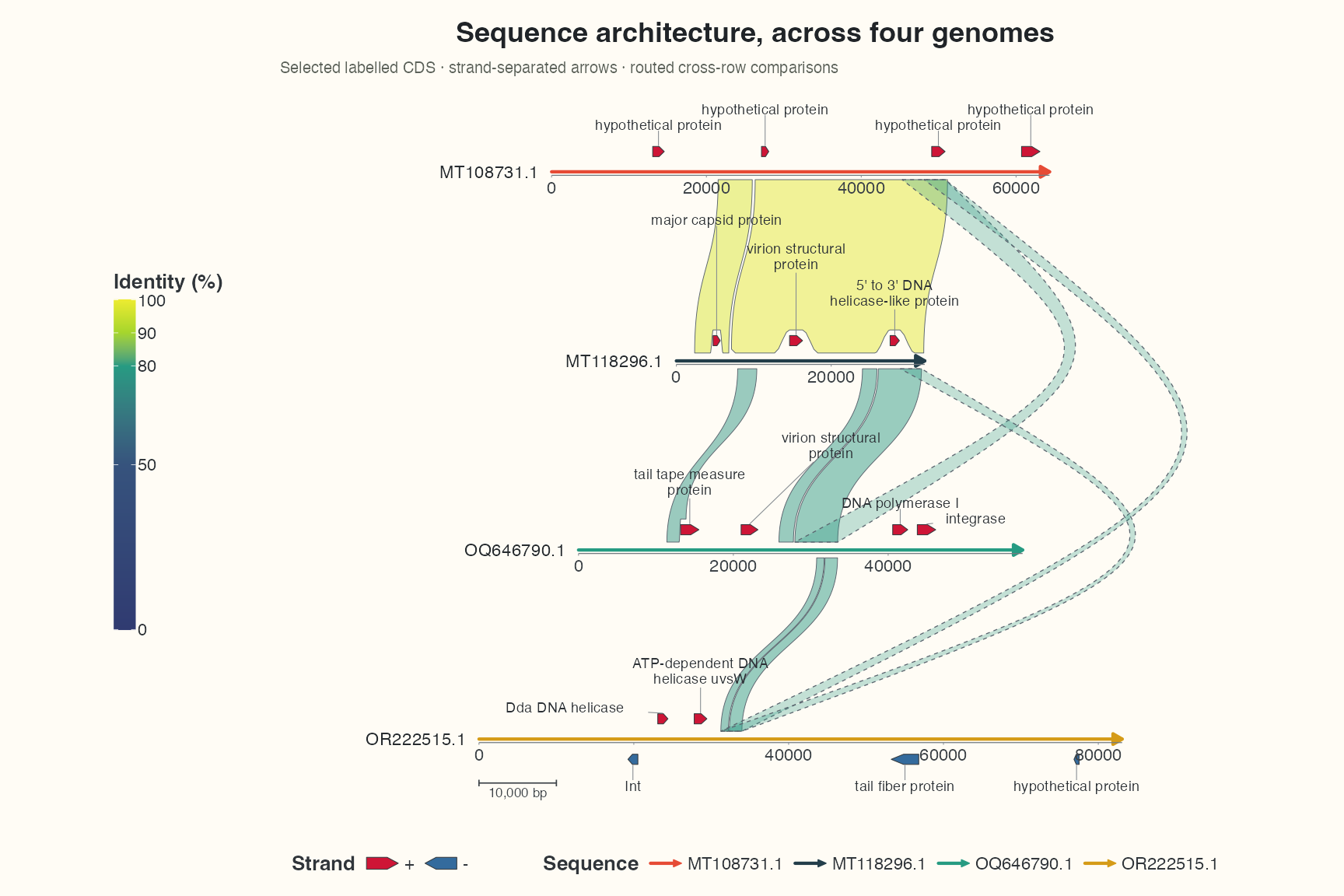
The linear showcase omits the crowded tail assembly protein and gp4 protein candidates, retaining them in the source and chord view; the remaining 16 features are individually labelled. Keep the selected adjacent HSPs and one longest HSP per non-neighbour pair. show_cross_controls matches show_cross row order; rebuild both after sorting/filtering. Controls use exported layout x/y units, not bp. Each link accepts two or four numbers, shaping its two ribbon edges rather than invoking a global route planner.
Shorter sequences are horizontally centred. A backbone-only layout provides actual row positions, lengths and offsets; controls are placed just beyond the intervening right ends rather than far from the data. Row spacing uses seq_gap and the longest backbone width, while controls do not accept bp coordinates. Changing spacing, order or orientation requires inspecting the paths again; arbitrary controls are not guaranteed free of self-intersection.
Local clearance and dashed outlines
position_strand() separates strands. link_avoid = "smooth" with the default NULL gap retreats locally near arrows. Non-adjacent outlines are dashed by default; a larger linewidth makes them visible without overriding linetype. Adjacency follows display order, not biological alignment direction.
Why the ruler was offset
geom_seq_scale() defaults to a 2 mm horizontal and 6 mm vertical offset. The earlier inset was configuration, not incorrect bp conversion. offset = unit(c(0, 10), "mm") aligns the start with the left sequence envelope and reserves vertical label space. With centred rows, source coordinate0 is no longer aligned across sequences; the ruler uses the left envelope, and reversed rows have their source origin at the other end. A scale bar measures distance rather than a particular source interval.
Continue in depth
Use focus/segments for local questions and CDS neighbourhoods for homology evidence; review the 2.6 Showcase. GC remains available in tracks, while the flagship reserves space for labels and links.