0.16.6 documentation

Site guide · find your task

Setup and learning paths

HomeInstall and prepare the environmentChoose your learning module

Module I · Chord

1.1 Tables and field meanings1.2 Produce and import comparisons1.3 Build the layers step by step1.4 Direction, curvature and clearance1.5 Filter and summarize links1.6 Full source-file workflow1.7 Complete chord showcase

Module II · Collinear

2.1 Reuse chord input tables2.2 Switch coordinates and add layers2.3 Routes, clearance and the ruler2.4 Compare CDS neighbourhoods2.5 Focus, anchors and segments2.6 Complete collinear showcase

Module III · Plasmid

3.1 DNA, annotations and 13 references3.2 From a circle to annotation layers3.3 Features, primers and restriction3.4 Thirteen plasmid references3.5 Complete plasmid cases

Consult as needed · Data and layers

Prepare tables and coordinatesImport and convert dataImport nucleotide and protein alignmentsProject protein intervals to genomic coordinatesFeatures, stacking and genomic decorationLabels and local placementQuantitative tracksMappings, scales, guides and themesSet values by sequence and strandCommon adjustments and grammarExport, preview and diagnostics

Learning map and reference

Articles and complete workflowsFunction referenceReproducible galleryFrequently asked questionsMigrate to the candidate APITerminology and design sourcesDevelopment status and changes

1.4 Direction, curvature and clearance

On this page

• Inspect directional evidence first
• Inspect directional evidence
• Combine capabilities into a readable view
• Why clearance modes look different
• Guides and export

These controls have different owners: geoms configure sequence geometry, Positions place local features, coords select the global view, and scales/guides control encodings.

Inspect directional evidence first

Extract the input bundle first.

Preparation code — run once on this page

Code

# Optional appearance choices; none of these columns or scales is required input.
library(ggchord)
seq_palette <- setNames(
  c("#E64B35", "#233E4A", "#269B82", "#D59B17"),
  c("MT108731.1", "MT118296.1", "OQ646790.1", "OR222515.1")
)
gene_palette <- c("+" = "#CE1536", "-" = "#346B9D", "." = "#8291A6")

library(ggchord)
doc_background <- "#FFFCF5"
identity_palette <- c("#303B71", "#36537D", "#269B82", "#A5D52C", "#ECEB31")
identity_values <- c(0, 0.5, 0.8, 0.9, 1)
identity_breaks <- c(0, 50, 80, 90, 100)
doc_legend_theme <- theme(
  legend.title = element_text(size = 13, face = "bold"),
  legend.text = element_text(size = 11),
  legend.key.width = unit(9, "mm"), legend.key.height = unit(5, "mm"),
  legend.spacing.x = unit(9, "mm"), legend.spacing.y = unit(7, "mm"),
  legend.margin = margin(l = 4, r = 4, unit = "mm")
)
sequence_guide <- guide_ggchord_legend(nrow = 1, theme = doc_legend_theme)
strand_guide <- guide_ggchord_legend(
  nrow = 1, override.aes = list(strand = c("+", "-")), theme = doc_legend_theme
)
identity_guide <- guide_ggchord_colourbar(
  position = "left", direction = "vertical",
  theme = theme(
    legend.key.height = unit(75, "mm"), legend.key.width = unit(5, "mm"),
    legend.title = element_text(size = 13, face = "bold"),
    legend.text = element_text(size = 11), legend.margin = margin(r = 7, unit = "mm")
  )
)
doc_theme <- theme_ggchord_publication(
  axis.text = element_text(size = 11),
  axis.text.check.overlap = TRUE
) +
  theme(
    legend.position = "bottom",
    legend.title = element_text(size = 13, face = "bold"),
    legend.text = element_text(size = 11),
    legend.key.width = unit(9, "mm"), legend.key.height = unit(5, "mm"),
    legend.spacing.x = unit(9, "mm"), legend.spacing.y = unit(7, "mm"),
    legend.box.spacing = unit(6, "mm"),
    plot.background = element_rect(fill = doc_background, colour = NA),
    panel.background = element_blank(),
    plot.title = element_text(face = "bold", size = 18),
    plot.subtitle = element_text(size = 10, colour = "#5C625A"),
    plot.margin = margin(14, 18, 14, 18)
  )
doc_axis <- function(coordinates = "relative") {
  scale_seq_position_continuous(
    coordinates = coordinates, n.breaks = 3, minor_breaks = NULL,
    labels = function(x) format(x, scientific = FALSE, big.mark = ",", trim = TRUE)
  )
}

library(ggchord)
library(dplyr)
library(purrr)
library(tidyr)
# Original repository records; extract the tutorial input bundle first.
show_sequences <- read_fasta_lengths(files = "examples/fasta/*.fna") |>
  select(accver, length)
show_annotations <- read_gff3(files = "examples/gff3/*.gff3", unstranded = "keep")
show_genes <- show_annotations |>
  filter(type == "CDS") |>
  select(accver, start, end, strand, anno)
show_alignments <- read_blast(files = "examples/blastn-standard/*.tsv")
# At most three substantial observed HSPs per pair; no coordinates are invented.
show_links <- show_alignments |>
  filter(length >= 900, pident >= 75) |>
  group_by(qaccver, saccver) |>
  slice_max(length, n = 3, with_ties = FALSE) |>
  ungroup()
# Select up to four source CDS per sequence, spread across annotation order.
# No feature is moved or invented; keep complete source tables separately.
show_features <- show_genes |>
  filter(end - start + 1 >= 500) |>
  group_by(accver) |>
  arrange(start, .by_group = TRUE) |>
  mutate(display_bin = ntile(row_number(), 4), informative = !is.na(anno) & anno != "hypothetical protein") |>
  group_by(accver, display_bin) |>
  arrange(desc(informative), desc(end - start), .by_group = TRUE) |>
  slice_head(n = 1) |>
  ungroup() |>
  select(accver, start, end, strand, anno)
# Also retain well-separated negative-strand CDS, if not already represented.
show_reverse <- show_genes |>
  filter(strand == "-", end - start + 1 >= 500) |>
  group_by(accver) |>
  arrange(start, .by_group = TRUE) |>
  slice(c(1, n())) |>
  ungroup()
show_features <- bind_rows(show_features, show_reverse) |>
  distinct(accver, start, end, strand, .keep_all = TRUE) |>
  arrange(accver, start)
show_labels <- show_features
show_optimization <- optimize_ggchord_layout(
  show_sequences, show_links,
  optimize = "orientation", weight = "length"
)

Inspect directional evidence

show_optimization optimizes display orientation only, preserving sequence order and weighting observed alignment lengths. Inspect seq_orientation and score_before/score_after. A display flip is not a new biological inversion result; the heuristic does not guarantee a global optimum.

Combine capabilities into a readable view

Code

show_curvature <- c(
  "MT108731.1" = 0, "MT118296.1" = 0.85,
  "OQ646790.1" = 1.1, "OR222515.1" = -0.4
)
show_radius <- c(
  "MT108731.1" = 1, "MT118296.1" = 1.05,
  "OQ646790.1" = 0.95, "OR222515.1" = 1.08
)
p_show_chord <- ggchord(show_sequences, show_links, show_features) +
  geom_link_ribbon(aes(ribbon_fill = pident), link_avoid = "smooth", alpha = 0.58, linewidth = 0.18) +
  geom_seq(
    seq_orientation = show_optimization$seq_orientation,
    seq_curvature = show_curvature, seq_radius = show_radius,
    seq_gap = 0.06, linewidth = 1.1
  ) +
  geom_gene(position = position_strand(0.07), width = 0.035) +
  geom_gene_label_repel(
    data = show_labels, label_layout = "radial", label_wrap = 24,
    size = 3.1, label_max_lines = 3, position = position_strand(0.07)
  ) +
  geom_seq_label(size = 4, seq_label_radius = 0.84, seq_label_hjust = 0.5) +
  scale_seq_colour_manual(
    values = seq_palette, name = "Sequence",
    guide = sequence_guide
  ) +
  scale_gene_fill_manual(values = gene_palette, breaks = c("+", "-"), name = "Strand") +
  scale_ribbon_fill_gradientn(
    colours = identity_palette, values = identity_values,
    limits = c(0, 100), breaks = identity_breaks, name = "Identity (%)", guide = identity_guide
  ) +
  guides(gene_fill = strand_guide) +
  scale_seq_position_continuous(breaks = c(0, 20000, 40000), minor_breaks = NULL) +
  coord_chord(rotation = 50) +
  doc_theme +
  labs(
    title = "Four genomes, one connected view",
    subtitle = "Signed curvature and radius · selected strand-aware CDS · local ribbon clearance"
  )
p_show_chord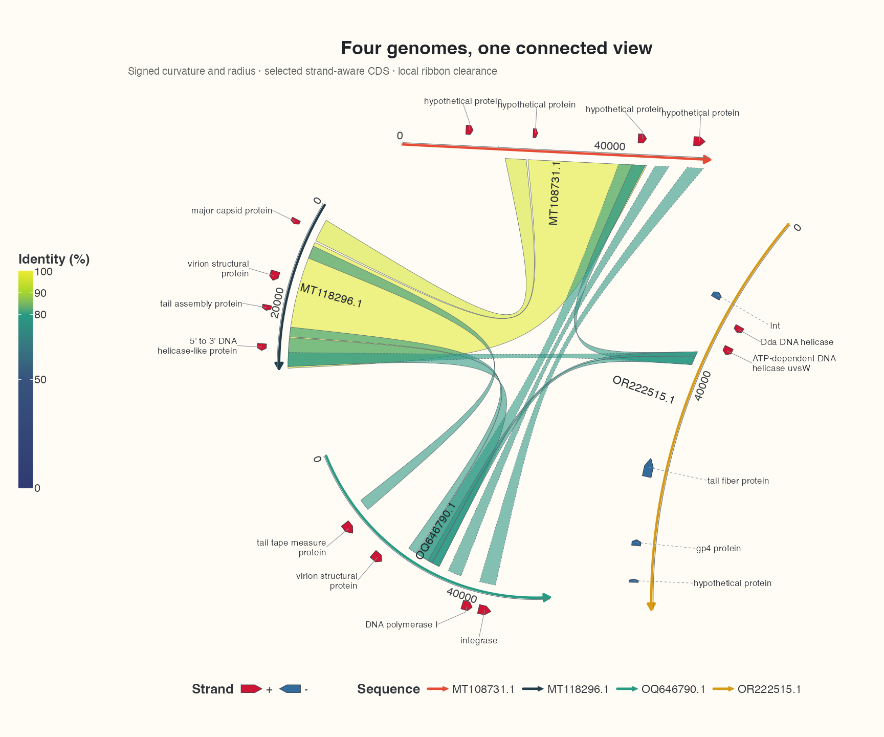

Four-genome chord comparison with mixed backbone curvature and measured identity · Click to enlarge

Named vectors match sequence IDs. Curvature 0 is straight, signed values bend in opposite directions, and magnitude changes bow depth. Radius changes sequence placement. The result combines automatic orientation, varying radius, zero/positive/negative curvature and local clearance without changing source coordinates.

Why clearance modes look different

link_avoid = "uniform" clears the whole endpoint interval. "smooth" retreats locally near feature polygons; "none" disables feature avoidance. Automatic clearance requires link_gap = NULL; a fixed number overrides it. Clearance considers feature geometry, not text, and does not automatically route around intervening sequence rows.

Guides and export

Identity uses a long left-side colourbar; sequence and strand keys remain below. Explicit strand overrides mirror the arrow glyphs. See styling for guide responsibilities. Save at 12×10 in, then review 1.7 The complete showcase.