Chapters and reference
Module IV · Multi-view composition · Section 5 of 6
4.4 Local magnification and character details
On this page
Data preparation and settings (expand)
R · Example code
library(dplyr)
fusion_hsp <- sequence_detail_example$paf
fusion_seqs <- bind_rows(
fusion_hsp |> transmute(accver = qaccver, length = qlen),
fusion_hsp |> transmute(accver = saccver, length = slen)
) |>
distinct()
fusion_colours <- setNames(c("#0072B2", "#D55E00"), fusion_seqs$accver)
fusion_links <- fusion_hsp |>
filter(length >= 900, pident >= 85)
fusion_events <- fusion_hsp |>
transmute(accver = qaccver, pos = qstart)R · Example code
fusion_center <- ggchord(fusion_seqs |> slice(1)) +
geom_seq(aes(seq_colour = accver), show.legend = FALSE) +
geom_track(
data = fusion_events, geom = "bar", stat = "bin", binwidth = 2000,
boundary = 1, closed = "left", bounds = "clip",
track = position_track("hsp-start-count", width = unit(6, "mm"))
) +
scale_track_value_continuous("hsp-start-count", name = NULL, breaks = c(0, 5)) +
scale_seq_colour_manual(values = fusion_colours) +
coord_circular()R · Example code
fusion_linear <- ggchord(fusion_seqs, fusion_hsp) +
geom_seq(show.legend = FALSE) +
geom_link_ribbon(show.legend = FALSE) +
geom_seq_label() +
scale_seq_colour_manual(values = fusion_colours) +
coord_collinear()
fusion_vertical <- fusion_linear +
coord_collinear(seq_axis = "vertical")R · Example code
p_fusionview <- ggchord_fusion(fusion_center, layout = "adaptive") +
fusion_panel(fusion_vertical, id = "detail", side = "right") +
fusion_ribbon(fusion_links, qpanel = "center", spanel = "detail", alpha = 0.28)1 A source interval and its local detail
magnify_ggchord() composes a Circular/Chord/Collinear source and an explicit Collinear or registered character detail plot. A source interval is biological data, not a rectangle in image pixels. The same region must be fully visible in both panels. Both rebuild at the final device size; no screenshot is stretched.
This example selects pETDuet-1 source positions 101–1900 (1800 bp). Its origin-crossing annotation at 5404→2 has no overlap with this interval; exclude it explicitly before linear focusing rather than taking its min/max as a long feature. The detail retains 10 annotations and labels the explicitly selected CDS/replication-origin subset. Reversing the detail’s display orientation changes neither source coordinates nor biological strands.
R · Example code
plasmid <- plasmid_example_pETDuet_1
annotations <- find_common_features(plasmid)
selected_region <- data.frame(accver = plasmid$accver, start = 101, end = 1900)
local_source <- focus_ggchord_data(
plasmid,
feature_data = annotations |> filter(start <= end),
loci = selected_region
)
whole_plasmid <- ggchord(plasmid, feature_data = annotations) +
geom_seq(show.legend = FALSE) +
geom_feature(position = position_plasmid(), show.legend = FALSE) +
geom_seq_center_label() +
coord_circular(rotation = -30)
local_labels <- local_source$feature_data |>
filter(type %in% c("CDS", "rep_origin"), anno != "ATG")
local_detail <- ggchord(
local_source$seq_data, feature_data = local_source$feature_data
) +
geom_seq(seq_orientation = -1, show.legend = FALSE) +
geom_feature(show.legend = FALSE) +
geom_feature_label(
data = local_labels, label_orientation = "horizontal",
label_overlap = "allow", colour = "#202020", size = 3
) +
coord_collinear(seq_axis = "vertical") +
scale_seq_position_continuous(coordinates = "source")
focused_view <- magnify_ggchord(whole_plasmid, selected_region, local_detail)
focused_view
focus_geometry <- export_ggchord_fusion(focused_view, width = 12, height = 8)
focus_geometry$focus_regions
focus_geometry$leaders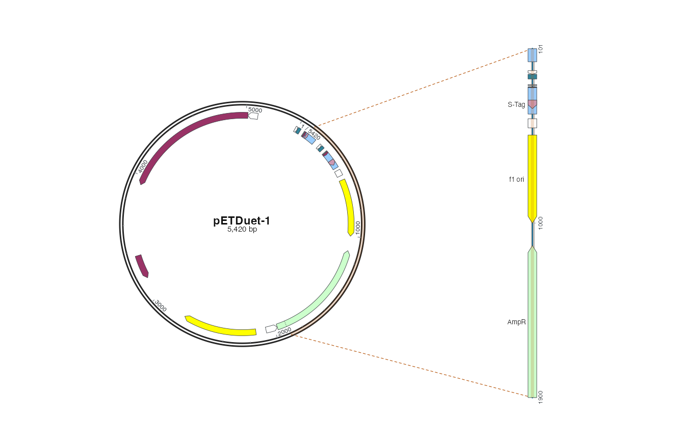
Use ordinary ggsave() at a chosen physical size, for example 12×8 inches; view_ggchord() uses the same renderer. center_size and detail_size are container fractions, while highlight_width is physical mm. Changing the detail side or orientation can change leader crossings; global collision avoidance is not claimed. connector = "none" keeps only highlights.
1.1 Source frame and selected zoom interval
By default the source frame uses the exact horizontal source coordinates in region; construct the explicit detail plot for the same interval. highlight_width independently controls physical frame height in millimetres, so vertical layout need not match the detail. Use frame_region to change only the frame: provide one ordered start/end row per region, in matching order. The real region, detail data and measured magnification ratio retain their original values. Frames must be fully visible in the same source instance; split origin-wrapping overrides explicitly.
R · Example code
source_frame <- selected_region |>
mutate(start = start - 20, end = end + 20)
framed_view <- magnify_ggchord(whole_plasmid, selected_region, local_detail,
frame_region = source_frame, highlight_width = 1.5)
export_ggchord_fusion(framed_view, width = 12, height = 7)$focus_regions |>
select(accver, start, end, frame_start, frame_end)The selected zoom interval remains 101–1900, while the source frame becomes 81–1920. Exported start/end and frame_start/frame_end distinguish them; focus_frame_region_data retains the original frame settings separately. Character panels use unfilled cell outlines so translucent highlights do not obscure letters or residue colours.
The dashed lines are decorative focus leaders. They are exported separately from biological connections and relationship_data; adding actual fusion_ribbon() layers still requires real relationship data. focus_region_data preserves the original selection and arbitrary metadata, while focus_regions reports resolved instances, source origins and the sampled physical path-length ratio. The ratio can be below one with a small detail allocation; it is not a change to biological length.
The detail plot owns its data, scales, layers and statistics. For count/bin/coverage tracks, prepare and state the intended local or global statistical population yourself; the wrapper records explicit_detail_plot and never silently chooses a scope. It does not copy arbitrary source layers, infer alignments or accept unregistered Cartesian character panels. Use one ordered region, explicitly select instance/detail_instance when an accession is repeated, and declare wrap = TRUE for origin-crossing selections as described below. Explicit nested/free-position allocations are described below; measured obstacle routing is described below.
2 Paired source windows with real HSPs
In this example, each row of region selects one original source interval; all rows share one explicit detail panel. The example selects the two endpoints of a real HSP from the four-sequence dataset. Gene direction and the local HSP come from the focused input tables. region_row links each derived region, front and decorative leader to its input row; arbitrary original metadata stays in focus_region_data.
R · Example code
library(dplyr)
seqs <- seq_data_example |> select(accver, length)
features <- gene_data_example |> mutate(strand = source_strand, type = 'CDS')
hsp <- ribbon_data_example |> slice(1)
regions <- bind_rows(
transmute(hsp, accver = qaccver, start = pmin(qstart, qend), end = pmax(qstart, qend)),
transmute(hsp, accver = saccver, start = pmin(sstart, send), end = pmax(sstart, send))
)
local <- focus_ggchord_data(seqs, feature_data = features,
ribbon_data = hsp, loci = regions)
source <- ggchord(seqs, feature_data = features, ribbon_data = hsp) +
geom_seq(show.legend = FALSE) + geom_gene(show.legend = FALSE) +
geom_link_ribbon(show.legend = FALSE)
detail <- ggchord(local$seq_data, feature_data = local$feature_data,
ribbon_data = local$ribbon_data) + geom_seq(show.legend = FALSE) +
geom_gene(show.legend = FALSE) + geom_link_ribbon(show.legend = FALSE) + coord_collinear()
paired_detail <- magnify_ggchord(
source + coord_collinear(), regions, detail, side = "bottom"
)
paired_detail
export_ggchord_fusion(paired_detail, width = 12, height = 8)$focus_regions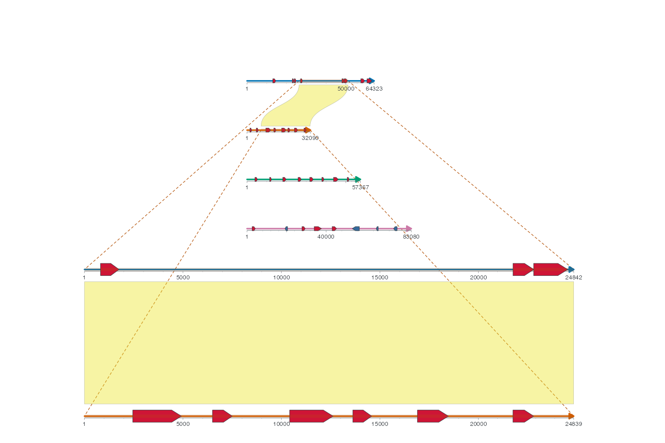
This does not create multiple insets or infer base-level alignments. Each interval must be fully visible in both panels. Instance selectors apply per row.
3 Independent detail panels
Split the two endpoints of one real HSP into independent local views. A named list supplies the detail plots, detail_panel routes each source row, and a named side vector assigns distinct sides. Each panel owns its data and scales.
R · Example code
library(ggchord)
library(dplyr)
seqs <- seq_data_example |> select(accver, length)
hsp <- ribbon_data_example |> slice(1)
regions <- bind_rows(
transmute(hsp, accver = qaccver, start = pmin(qstart, qend),
end = pmax(qstart, qend), detail_panel = "query"),
transmute(hsp, accver = saccver, start = pmin(sstart, send),
end = pmax(sstart, send), detail_panel = "subject")
)
make_detail <- function(region) {
local <- focus_ggchord_data(seqs, loci = region)
ggchord(local$seq_data) +
geom_seq(show.legend = FALSE) +
coord_collinear(seq_axis = "vertical")
}
source <- ggchord(seqs, hsp) +
geom_seq(show.legend = FALSE) +
geom_link_ribbon(show.legend = FALSE)
details <- list(
query = make_detail(regions[1, ]),
subject = make_detail(regions[2, ])
)
multiple <- magnify_ggchord(
source, regions, details,
side = c(query = "left", subject = "right")
)
export_ggchord_fusion(multiple, width = 12, height = 8)$focus_regions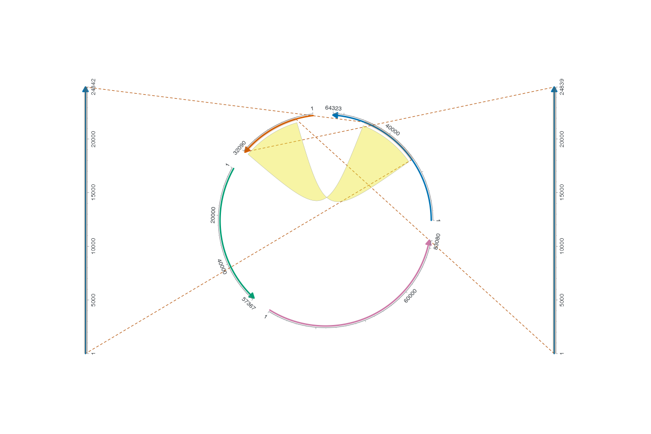
This example uses four named details, one per cardinal side; diagonal sides and explicit boxes are available below. Every panel needs a region; missing or unknown targets fail. Source and detail instance selectors remain independent. detail_size accepts a named list of width/height fractions; NULL uses Fusion defaults. Overlaps fail rather than displacing explicit allocations. Standard saving rebuilds panels and leaders at the requested size. At small sizes, inspect labels and enlarge the canvas as needed. Leaders may cross the main plot or one another; global avoidance is separate from the explicit nested/box allocation described below.
4 Character details with exact source anchors
An ordinary Cartesian character plot becomes an independent detail panel through register_ggchord_alignment(). Register the displayed cells: x is the original alignment/coding column, y is the alignment-row ID and label is the observed character. Source mapping remains independent of ordinary ggplot scales. This actual 30-column excerpt preserves upstream gaps and mismatches; macro lengths describe ungapped alignment fragments, not complete genomes. Short labels affect display only; original record IDs remain intact.
R · Example code
library(dplyr)
cells <- sequence_detail_example$dna_alignment
rows <- unique(cells$accver)[c(1, 3)]
window <- cells |>
  filter(accver %in% rows, between(alignment_column, 321, 350))
sequences <- cells |>
  filter(accver %in% rows, !is_gap) |>
  group_by(accver) |>
  summarise(length = max(source_position), .groups = "drop")
regions <- window |>
  filter(!is_gap) |>
  group_by(source_accver) |>
  summarise(start = min(source_position), end = max(source_position), .groups = "drop") |>
  rename(accver = source_accver)
letters <- ggplot2::ggplot(window, aes(alignment_column, accver, label = symbol)) +
  geom_residue(overflow = "error", show.legend = FALSE) +
  ggplot2::scale_y_discrete(limits = rev(rows),
    labels = setNames(c("AF191661.1", "AF191659.1"), rows),
    expand = expansion(add = 0.6)) +
  ggplot2::scale_x_continuous(breaks = seq(321, 350, 5), expand = expansion(add = 0.6)) +
  labs(title = "Aligned nucleotide detail", x = "Alignment column", y = NULL) +
  ggplot2::theme_minimal(base_size = 12) +
  theme(panel.grid = element_blank(), plot.title = element_text(face = "bold"),
    axis.text = element_text(colour = "#25363B"))
letters <- register_ggchord_alignment(letters, window)
macro <- ggchord(sequences) +
  geom_seq(aes(seq_colour = accver), show.legend = FALSE) +
  geom_seq_label(labels = setNames(c("AF191661.1", "AF191659.1"), rows), size = 3.5) +
  coord_collinear() +
  labs(title = "Sequence context") +
  theme_ggchord_publication()
character_detail <- magnify_ggchord(
  macro, regions, letters,
  center_box = c(.01, .28, .20, .85), detail_box = c(.33, .99, .15, .85),
  connector = "envelope", colour = "#725094", highlight_width = 3
)
export_ggchord_fusion(character_detail, width = 16, height = 5)$focus_regions
# ggsave("character-detail.png", character_detail, width = 16, height = 5)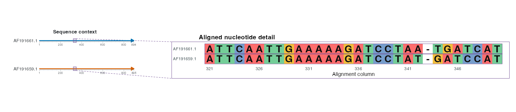
The ordinary plot remains editable: local colours, layers and annotations remain independent. Identity/reverse x scales and discrete y rows are supported. Each Fusion build verifies the registered residue positions/labels after edits and remeasures the final panel in mm; half-cell boundaries attach to the exact endpoint cells. Gap cells have no source position and are never interpolated into bases. A source interval must contain every selected base in biological order; split introns into separate source rows; origin joins use the explicit wrapping declaration below. Use detail_instance to select an alignment row when several rows share a source. Unregistered ggplots, facets, nonlinear/flipped coordinates and moved registered cells fail.
translate_ggchord_cds() nucleotide rows can be registered in the same way. Keep the translation on codon centres as in examples/m2-detail.R; use source_positions for full codon membership across segments. AA residue rows use their own aa coordinate domain; connecting a genomic bp macro directly to aa positions still requires an explicit CDS projection. Decorative magnify leaders remain separate from biological Fusion links. Character endpoints have no backbone colour for a Fusion gradient: supply explicit cross-panel fill. Narrow panels retain geom_residue()’s tile/error policy; enlarge the physical export instead of relying on DPI. Global leader avoidance is separate; explicit nested/free-position allocation is supported below.