Chapters and reference
Module IV · Multi-view composition · Section 6 of 6
4.5 Nested composition and origin-crossing zoom
On this page
Data preparation and settings (expand)
R · Example code
library(dplyr)
fusion_hsp <- sequence_detail_example$paf
fusion_seqs <- bind_rows(
fusion_hsp |> transmute(accver = qaccver, length = qlen),
fusion_hsp |> transmute(accver = saccver, length = slen)
) |>
distinct()
fusion_colours <- setNames(c("#0072B2", "#D55E00"), fusion_seqs$accver)
fusion_links <- fusion_hsp |>
filter(length >= 900, pident >= 85)
fusion_events <- fusion_hsp |>
transmute(accver = qaccver, pos = qstart)R · Example code
fusion_center <- ggchord(fusion_seqs |> slice(1)) +
geom_seq(aes(seq_colour = accver), show.legend = FALSE) +
geom_track(
data = fusion_events, geom = "bar", stat = "bin", binwidth = 2000,
boundary = 1, closed = "left", bounds = "clip",
track = position_track("hsp-start-count", width = unit(6, "mm"))
) +
scale_track_value_continuous("hsp-start-count", name = NULL, breaks = c(0, 5)) +
scale_seq_colour_manual(values = fusion_colours) +
coord_circular()R · Example code
fusion_linear <- ggchord(fusion_seqs, fusion_hsp) +
geom_seq(show.legend = FALSE) +
geom_link_ribbon(show.legend = FALSE) +
geom_seq_label() +
scale_seq_colour_manual(values = fusion_colours) +
coord_collinear()
fusion_vertical <- fusion_linear +
coord_collinear(seq_axis = "vertical")R · Example code
p_fusionview <- ggchord_fusion(fusion_center, layout = "adaptive") +
fusion_panel(fusion_vertical, id = "detail", side = "right") +
fusion_ribbon(fusion_links, qpanel = "center", spanel = "detail", alpha = 0.28)1 Nested source regions retain their own namespaces
A detail may itself be a Fusion. This example uses two explicit windows on the unchanged pUC19 source. The inner source is the larger window; its child is the smaller window. The outer selection targets the inner source through detail/center, not an arbitrary rectangle in an image.
R · Example code
data(plasmid_example_pUC19)
source_genome <- plasmid_example_pUC19 |>
dplyr::select(accver, length)
large_region <- data.frame(accver = "pUC19", start = 101, end = 1900)
small_region <- data.frame(accver = "pUC19", start = 301, end = 600)
large_window <- focus_ggchord_data(source_genome, loci = large_region)
small_window <- focus_ggchord_data(source_genome, loci = small_region)
large_plot <- ggchord(large_window$seq_data) +
geom_seq(show.legend = FALSE) + coord_collinear()
small_plot <- ggchord(small_window$seq_data) +
geom_seq(show.legend = FALSE) + coord_collinear()
inner <- magnify_ggchord(large_plot, small_region, small_plot)
whole <- ggchord(source_genome) + geom_seq() + coord_circular()
large_region$detail_panel <- "detail/center"
outer <- magnify_ggchord(
whole, large_region, inner,
center_box = c(.02, .22, .15, .85), detail_box = c(.27, .99, .1, .9)
)
report <- export_ggchord_fusion(outer, width = 14, height = 7)
report$focus_regions
report$focus_region_data_by_composition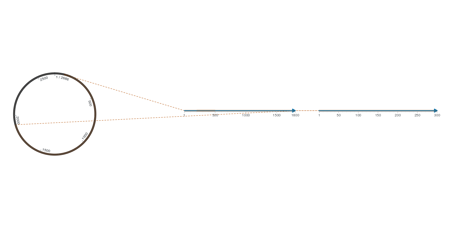
composition_id plus region_row connects derived regions/fronts/leaders to each original selection in focus_region_data_by_composition. Top-level focus_region_data remains the original outer input. Nested leaf names use paths such as detail/center and detail/detail; a composition container is never treated as one genomic axis. If an accession occurs in multiple leaves, select the full panel path and exact instance. source_panel can select a source leaf under center. Layout exports include actual mm boundaries and requested boxes/angles.
Each plot keeps its own layers, scales and statistical population; the compositor does not silently copy layers or recompute statistics. Origin wraps use the explicit source-length declaration below. The complete negative-strand CDS-to-genome-focus-to-real-character example is in examples/m3-nested.R. Registered characters retain their physical tile/error policy; a small nested allocation cannot make 60 letters readable merely by increasing DPI. Full multi-device publication acceptance and broader layout optimisation remain separate concerns.
2 Explicit origin-crossing selection
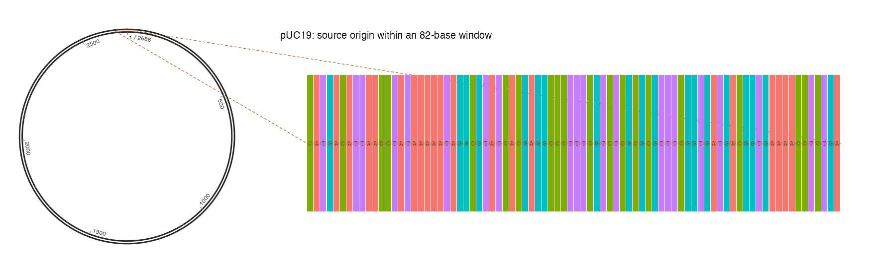
Circular layout is not evidence of a circular source. Set wrap = TRUE on a selection with start > end. Both selected leaf panels must retain the same full source length. Character adapters additionally require circular = TRUE and source_data with a full sequence or an exact source_length; without the full string, characters remain unverified. At most one source tour is allowed, so inverse source-to-column mapping stays unique. Negative strands wrap in their own direction and retain gaps. Different focused instances are never joined implicitly.
Run the complete real pUC19 workflow in examples/origin-detail.R. It extracts 82 observed bases (2640–2686, then 1–35) from the unchanged bundled FASTA. focus_region_data retains the original single row. Derived tables identify two pieces with region_piece, sharing one region_row; only the two external boundaries receive leaders. The seam is not another selection or relationship.
R · Example code
# Optional dependency: dplyr. Source: unchanged bundled pUC19 FASTA.
library(ggchord)
library(dplyr)
genome <- sequence_detail_example$plasmid_source
source_length <- genome$length[[1L]]
region <- tibble(accver = genome$accver, start = source_length - 46,
end = 35, wrap = TRUE)
# Extract actual source characters, keeping their order across the origin.
positions <- c(seq.int(region$start, source_length), seq_len(region$end))
fragment <- paste0(substring(genome$sequence, positions, positions), collapse = '')
source <- tibble(accver = 'origin-window', source_accver = genome$accver,
start = region$start, strand = '+', sequence = genome$sequence)
cells <- as_ggchord_alignment(c('origin-window' = fragment), 'DNA',
source_data = source, circular = TRUE)
characters <- ggplot2::ggplot(cells, aes(alignment_column, accver, label = symbol)) +
geom_residue(aes(fill = symbol), show.legend = FALSE) +
ggplot2::theme_void() +
ggplot2::labs(title = 'pUC19: source origin within an 82-base window')
characters <- register_ggchord_alignment(characters, cells)
whole <- ggchord(genome) + geom_seq(show.legend = FALSE) + coord_circular()
origin_detail <- magnify_ggchord(whole, region, characters,
center_box = c(.01, .28, .05, .95), detail_box = c(.32, .99, .1, .9))
view_ggchord(origin_detail, width = 16, height = 5, units = "in")