Chapters and reference
Module IV · Multi-view composition · Section 3 of 6
4.2 Cross-panel links and routing
On this page
Data preparation and settings (expand)
R · Example code
library(dplyr)
fusion_hsp <- sequence_detail_example$paf
fusion_seqs <- bind_rows(
fusion_hsp |> transmute(accver = qaccver, length = qlen),
fusion_hsp |> transmute(accver = saccver, length = slen)
) |>
distinct()
fusion_colours <- setNames(c("#0072B2", "#D55E00"), fusion_seqs$accver)
fusion_links <- fusion_hsp |>
filter(length >= 900, pident >= 85)
fusion_events <- fusion_hsp |>
transmute(accver = qaccver, pos = qstart)R · Example code
fusion_center <- ggchord(fusion_seqs |> slice(1)) +
geom_seq(aes(seq_colour = accver), show.legend = FALSE) +
geom_track(
data = fusion_events, geom = "bar", stat = "bin", binwidth = 2000,
boundary = 1, closed = "left", bounds = "clip",
track = position_track("hsp-start-count", width = unit(6, "mm"))
) +
scale_track_value_continuous("hsp-start-count", name = NULL, breaks = c(0, 5)) +
scale_seq_colour_manual(values = fusion_colours) +
coord_circular()R · Example code
fusion_linear <- ggchord(fusion_seqs, fusion_hsp) +
geom_seq(show.legend = FALSE) +
geom_link_ribbon(show.legend = FALSE) +
geom_seq_label() +
scale_seq_colour_manual(values = fusion_colours) +
coord_collinear()
fusion_vertical <- fusion_linear +
coord_collinear(seq_axis = "vertical")R · Example code
p_fusionview <- ggchord_fusion(fusion_center, layout = "adaptive") +
fusion_panel(fusion_vertical, id = "detail", side = "right") +
fusion_ribbon(fusion_links, qpanel = "center", spanel = "detail", alpha = 0.28)1 Connect real source intervals
Fusion combines independent genomic plots and connects their real sequence intervals. The center and peripherals can use registered genomic Coord views; Sankey and Radial retain their explicit display instances. Nested Fusions and registered character details are supported. Each plot remains usable on its own. The composition rebuilds all panels at their actual physical sizes before drawing links.
This example uses bundled sequence_detail_example$paf; provenance of the original EMALE PAF is available on the input downloads and sources page. Data preparation requires optional dplyr. The PAF contains 11 observed HSPs; below we explicitly select the two with length ≥900 and Identity ≥85% for cross-panel display. The count track bins all original query-start observations into explicit 2,000 bp intervals and does not represent coverage depth. The last display bin is clipped to the true sequence boundary; source observations and counts are retained.
R · Example code
library(dplyr)
fusion_hsp <- sequence_detail_example$paf
fusion_seqs <- bind_rows(
fusion_hsp |> transmute(accver = qaccver, length = qlen),
fusion_hsp |> transmute(accver = saccver, length = slen)
) |>
distinct()
fusion_colours <- setNames(c("#0072B2", "#D55E00"), fusion_seqs$accver)
fusion_links <- fusion_hsp |>
filter(length >= 900, pident >= 85)
fusion_events <- fusion_hsp |>
transmute(accver = qaccver, pos = qstart)Keep reverse endpoints as normalized by read_paf(). A constructor warning about descending endpoints does not mean they should be sorted. Prepare two independent plots; explicit sequence colours keep their accession meanings consistent. Local legends are hidden explicitly because their sequence colours are already visible and only the cross-panel Identity legend is needed here.
R · Example code
fusion_center <- ggchord(fusion_seqs |> slice(1)) +
geom_seq(aes(seq_colour = accver), show.legend = FALSE) +
geom_track(
data = fusion_events, geom = "bar", stat = "bin", binwidth = 2000,
boundary = 1, closed = "left", bounds = "clip",
track = position_track("hsp-start-count", width = unit(6, "mm"))
) +
scale_track_value_continuous("hsp-start-count", name = NULL, breaks = c(0, 5)) +
scale_seq_colour_manual(values = fusion_colours) +
coord_circular()R · Example code
fusion_linear <- ggchord(fusion_seqs, fusion_hsp) +
geom_seq(show.legend = FALSE) +
geom_link_ribbon(show.legend = FALSE) +
geom_seq_label() +
scale_seq_colour_manual(values = fusion_colours) +
coord_collinear()
fusion_vertical <- fusion_linear +
coord_collinear(seq_axis = "vertical")The fixed qpanel and spanel select the exact query and subject panels. The ribbon is anchored to the matching sequence in the multi-sequence panel, not its outer rectangle or center. Query/subject roles do not indicate a biological flow of genetic material.
R · Example code
p_fusionview <- ggchord_fusion(fusion_center, layout = "adaptive") +
fusion_panel(fusion_vertical, id = "detail", side = "right") +
fusion_ribbon(fusion_links, qpanel = "center", spanel = "detail", alpha = 0.28)
view_ggchord(p_fusionview, width = 11, height = 8, units = "in")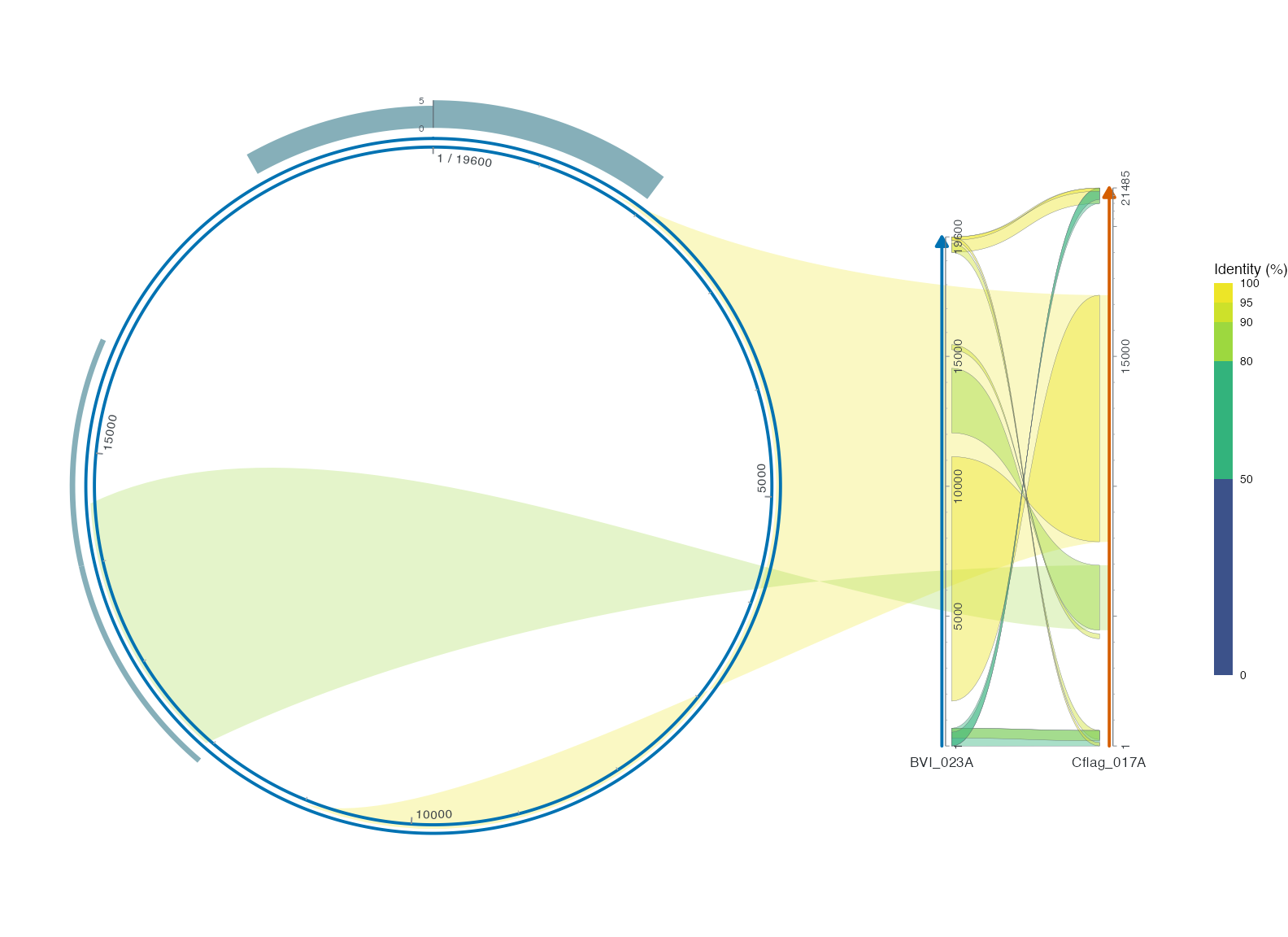
2 Register panels and instances
The first example uses one panel per named side: right, top, left, bottom. Diagonal, free and automatic placement are described below. IDs must be unique; center is reserved. size=c(width,height) and center_size are fractions of the content area after native outer decoration and cross-panel Guides have been allocated. Explicit allocations that overlap fail rather than silently relocating a panel. A side specifies placement; it does not rotate a plot’s text. Set the plot’s own coord_collinear(seq_axis="vertical") for a vertical sequence axis.
The four-direction example reuses source PAF rows 3, 2, 9 and 1, explicitly connecting them north, west, south and east. These repeated views are separate display instances, not extra observations. Different panels need not share a physical bp/mm scale.
R · Example code
p_fusionfour <- ggchord_fusion(fusion_center, layout = "adaptive") +
fusion_panel(fusion_vertical, id = "east", side = "right") +
fusion_panel(fusion_vertical, id = "west", side = "left") +
fusion_panel(fusion_linear, id = "north", side = "top") +
fusion_panel(fusion_linear, id = "south", side = "bottom") +
fusion_ribbon(fusion_hsp |> slice(3), qpanel = "center", spanel = "north", fill = "#0072B2") +
fusion_ribbon(fusion_hsp |> slice(2), qpanel = "center", spanel = "west", fill = "#0072B2") +
fusion_ribbon(fusion_hsp |> slice(9), qpanel = "center", spanel = "south", fill = "#0072B2") +
fusion_ribbon(fusion_hsp |> slice(1), qpanel = "center", spanel = "east", fill = "#0072B2", alpha = 0.16)
view_ggchord(p_fusionfour, width = 14, height = 11, units = "in")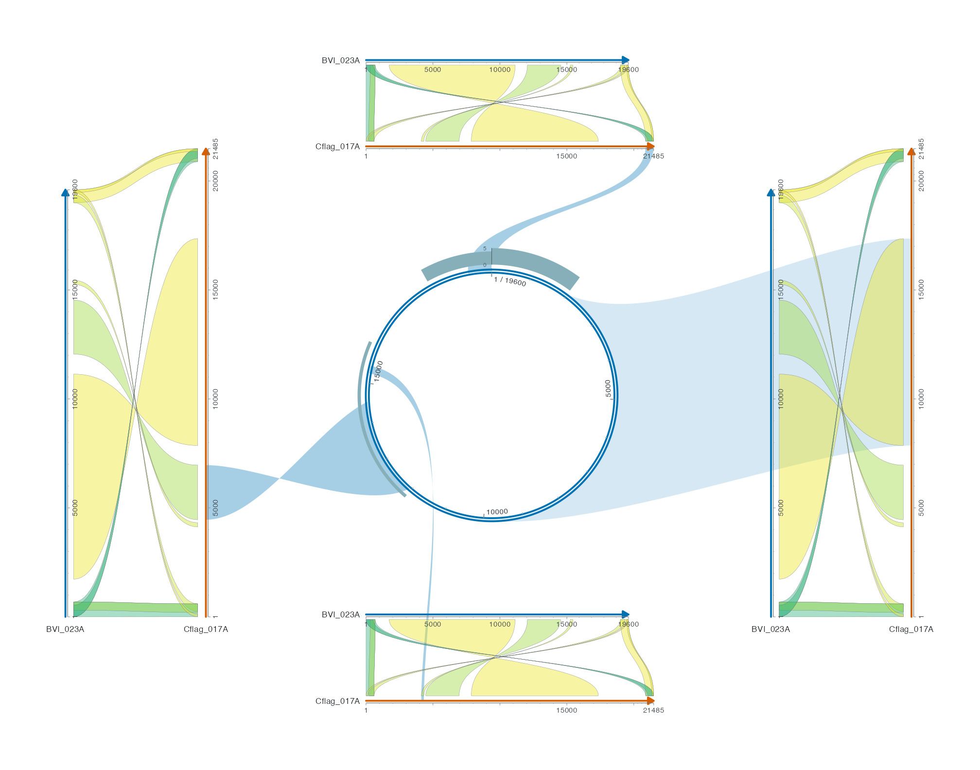
Selectors can also be columns qpanel, spanel, q_instance, s_instance. Do not provide both a fixed panel argument and its column. If an accession occurs in several panels or repeated display instances, omission is allowed only when exactly one fully visible interval matches. Ambiguity is an error; name the intended panel and instance. Original source coordinates also work for explicitly renamed focus windows via their retained source origins. Repeated source_hsp_id display requires allow_repeated=TRUE in every participating layer. Without IDs, source rows remain layer-local; identical values are not treated as a shared biological identity.
3 Export and inspect anchors
R · Example code
fusion_layout <- export_ggchord_fusion(p_fusionview, width = 11, height = 8)
fusion_layout$connections |>
select(layer_id, source_row, qpanel, q_instance, spanel, s_instance, retained)
fusion_layout$fronts |>
select(panel_id, accver, position_boundary, x, y) |>
slice_head(n = 4)panels records actual panel/container bounds in mm. connections retains original relationship columns, source rows and resolved routes; unknown directions are explicitly omitted and reported. fronts contains local coordinates, source interval boundaries, global mm and local tangent/normal vectors. paths adds the rendered connection geometry; source_layouts, source_data and relationship_data preserve their separate provenance. Diagnostics include local label visibility, fit results and guide dimensions; unmeasured global collisions are not reported as zero.
Intervals are one-based inclusive, with full boundaries [min(start,end)-1,max(start,end)] ordered by the original endpoint direction. A one-position interval retains nonzero width. This new composition rule does not rewrite legacy single-view ribbon geometry. Source positions, interval boundaries and mm coordinates are different quantities.
export_ggchord_fusion() measures on a temporary device and restores the previous device. Saving rebuilds on the actual output device, so font metrics may differ slightly while source coordinates remain unchanged. Use ordinary ggsave() or the shared preview; do not use ggplot_build() on a composition.
R · Example code
ggsave("fusion.png", p_fusionview, width = 11, height = 8, units = "in", dpi = 300)
view_ggchord(p_fusionview, width = 11, height = 8, viewer = "none")Fully visible intervals are required. Prepare partial windows or splits in the source workflow explicitly. Ordinary fusion_ribbon() inputs require prepared continuous intervals. For cross-origin selections, use the explicit magnify_ggchord() with region wrap = TRUE region workflow below, with matching complete source lengths. Direct bp↔︎aa links, Dotplot, facets and unregistered external plots remain unsupported. direct, avoid and bundle route against their documented measured obstacles; they do not guarantee a global optimum. Explicit derived views and placement are described below. Links may cross or pass through panel interiors; foreground annotations are retained, but arbitrary layouts are not guaranteed collision-free.
4 Measured routes and display corridors
fusion_ribbon(route = "avoid") keeps both complete interval fronts and their physical departure normals. It routes a narrow polygonal body around measured other leaf containers, native layer text, and final gtable guide/decoration cells. route_width is in mm and does not encode an alignment length or count. The default "direct" preserves the existing Bezier drawing and reports its collisions; it does not silently filter records.
Use route = "bundle" with an explicit character route_group column to share a corridor within one layer and ordered panel pair. Each source row still has its own front, colour/alpha and polygon. Shared-channel overpainting is not read support or another observation. Groups are user declarations; no cluster or relationship is inferred. Run the real three-HSP example:
R · Example code
# Optional dependency: dplyr. These are real bundled HSP records.
library(ggchord)
library(dplyr)
first_hit <- ribbon_data_example |> slice_head(n = 1)
channel_hits <- ribbon_data_example |>
filter(qaccver == first_hit$qaccver, saccver == first_hit$saccver) |>
mutate(route_group = 'explicit-display-channel')
# Shared corridors describe drawing; they do not aggregate biological evidence.
panel <- ggchord(seq_data_example) +
geom_seq(show.legend = FALSE) +
geom_seq_label(size = 3, seq_label_rotation = 90) +
coord_collinear(seq_axis = 'vertical') +
theme(ggchord.axis = element_blank())
composition <- ggchord_fusion(panel, center_box = c(.02, .28, .12, .88)) +
fusion_panel(panel, 'target', box = c(.72, .98, .12, .88)) +
fusion_panel(panel, 'obstacle', box = c(.4, .6, .22, .78))
routed <- composition +
fusion_ribbon(channel_hits, qpanel = 'center', spanel = 'target',
route = 'bundle', route_width = .8, fill = '#548CA0', alpha = .3)
view_ggchord(routed, width = 12, height = 8, units = "in")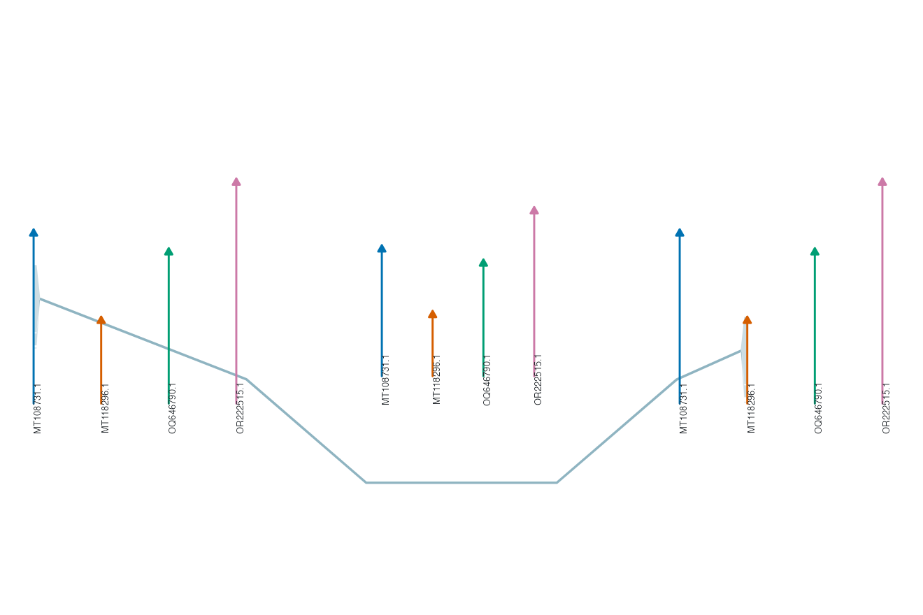
magnify_ggchord(route = "avoid") applies the same measured-space contract to its decorative leaders. Exported leader_paths contains the final polyline vertices, separate from biological paths. routing_corridors identifies shared channels and member source rows; routing_obstacles records the physical envelopes. Connections/leaders report route status and collisions. Each target size is rebuilt, including ancestor checks after nested allocation.
No clear route produces an explicit error: move/enlarge the panels, narrow a selection, revise a declared group, or inspect route = "direct". Ancestor overlays that obstruct an already measured child route also fail explicitly. Routing uses deterministic visibility paths, not a global layout optimum. Rotated text uses conservative bounding rectangles, curved strings larger envelopes, and native decoration cells their final gtable bounds. Arbitrary custom grobs and every endpoint data shape are not claimed to be glyph-level obstacles. Theme changes affect metrics, never source coordinates or evidence.