Chapters and reference
Module IV · Multi-view composition · Section 4 of 6
4.3 Panel placement, size and guides
On this page
See Flagship data sources and construction for provenance, display selections and rebuilding. This page loads bundled inputs directly and focuses on plotting settings.
Data preparation and settings (expand)
R · Example code
library(dplyr)
fusion_hsp <- sequence_detail_example$paf
fusion_seqs <- bind_rows(
fusion_hsp |> transmute(accver = qaccver, length = qlen),
fusion_hsp |> transmute(accver = saccver, length = slen)
) |>
distinct()
fusion_colours <- setNames(c("#0072B2", "#D55E00"), fusion_seqs$accver)
fusion_links <- fusion_hsp |>
filter(length >= 900, pident >= 85)
fusion_events <- fusion_hsp |>
transmute(accver = qaccver, pos = qstart)R · Example code
fusion_center <- ggchord(fusion_seqs |> slice(1)) +
geom_seq(aes(seq_colour = accver), show.legend = FALSE) +
geom_track(
data = fusion_events, geom = "bar", stat = "bin", binwidth = 2000,
boundary = 1, closed = "left", bounds = "clip",
track = position_track("hsp-start-count", width = unit(6, "mm"))
) +
scale_track_value_continuous("hsp-start-count", name = NULL, breaks = c(0, 5)) +
scale_seq_colour_manual(values = fusion_colours) +
coord_circular()R · Example code
fusion_linear <- ggchord(fusion_seqs, fusion_hsp) +
geom_seq(show.legend = FALSE) +
geom_link_ribbon(show.legend = FALSE) +
geom_seq_label() +
scale_seq_colour_manual(values = fusion_colours) +
coord_collinear()
fusion_vertical <- fusion_linear +
coord_collinear(seq_axis = "vertical")R · Example code
p_fusionview <- ggchord_fusion(fusion_center, layout = "adaptive") +
fusion_panel(fusion_vertical, id = "detail", side = "right") +
fusion_ribbon(fusion_links, qpanel = "center", spanel = "detail", alpha = 0.28)1 Styles and physical layout
Cross-panel layers accept aes(fill=..., colour=..., alpha=..., linewidth=..., linetype=...) with ordinary ggplot2 scales. Panel role-specific scales remain local. Explicit fixed styles override their mappings. Default Identity is 0–100 with 0/50/80/90/95/100 proportional breaks. Endpoint gradients and subject tips are opt-in, using the same renderer as single-view ribbons. A tip is a decorative direction marker; full source fronts remain exported.
R · Example code
fusion_gradient <- ggchord_fusion(fusion_center) +
fusion_panel(fusion_vertical, id = "detail") +
fusion_ribbon(
fusion_hsp |> slice(3), qpanel = "center", spanel = "detail",
gradient = TRUE, tip = "subject"
)
fusion_mapped <- ggchord_fusion(fusion_center) +
fusion_panel(fusion_vertical, id = "detail") +
fusion_ribbon(fusion_links, aes(fill = pident), qpanel = "center", spanel = "detail") +
ggplot2::scale_fill_gradient(low = "#3B528B", high = "#FDE725", limits = c(0, 100))Default layout="fixed" allocates panel rectangles and rebuilds their labels and guides at the output size. layout="adaptive" additionally fits the central rectangle to the physical aspect ratio and jointly budgets native outer Guides. Explicit font sizes remain fixed. This is not a general font-scaling or global collision solver. Each panel retains its own guides; different scale meanings are not automatically merged. Use show.legend=FALSE or local theme() deliberately where appropriate. Composition guides() configures cross-panel Guides; theme() also styles the native outer plot furniture described below. Required guide space is measured; a canvas too small for it fails with a diagnostic.
2 Eight directions and independent physical placement
fusion_panel() supports the four cardinal sides plus topright, topleft, bottomright and bottomleft. Default corner layouts reserve space for all eight; side names remain unique. For other arrangements use angle/distance or an explicit box. There is no fixed panel-count limit for explicit boxes/angles: every allocation must still fit. Placement changes the container, not the child’s Coord or text orientation. Angles describe physical directions on rectangular exports; distance is a fraction of half the shorter allocation dimension, measured from the centre allocation.
R · Example code
data(seq_data_example)
sequences <- seq_data_example |>
dplyr::select(accver, length)
base_panels <- ggchord(sequences) + geom_seq(show.legend = FALSE)
central <- base_panels + coord_chord()
mirrored <- base_panels + coord_sankey()
free_angle <- ggchord_fusion(central) +
fusion_panel(mirrored, "mirror", angle = 31, distance = .8, size = c(.16, .22))
free_box <- ggchord_fusion(central, center_box = c(.02, .35, .2, .8)) +
fusion_panel(mirrored, "mirror", box = c(.45, .98, .1, .9))
physical_box <- ggchord_fusion(central, center_box = unit(c(5, 85, 10, 100), "mm")) +
fusion_panel(mirrored, "mirror", box = unit(c(100, 210, 10, 100), "mm"))
export_ggchord_fusion(physical_box, width = 12, height = 6)$panels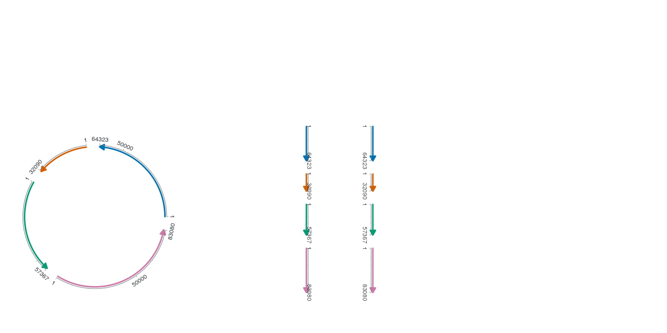
A numeric box uses xmin, xmax, ymin, ymax fractions; an absolute-unit box keeps its physical dimensions. Coordinates refer to the composition content area after native outer plot decorations and cross-panel Guides. Do not combine box with side/size/angle/distance, or center_box with center_size. Physical allocations are checked at every target size; they are never silently clamped. Explicit allow_overlap = TRUE on ggchord_fusion() or magnify_ggchord() permits deliberate overlays. Later panels cover earlier panels, using vector grid clipping rather than PNG crops; translucent connections are not repainted twice in the same area. The export’s overlaps table records covering order. This permits intentional masks and does not promise automatic obstacle avoidance.
Sankey source IDs occur in both mirrored columns. Choose an exact q_instance/s_instance from get_chord_layout(plot)$display_instances; omission fails when ambiguous. Radial and Chord use their own registered backbone frames. All q/s intervals, units and source records remain unchanged. If a declared source_hsp_id appears repeatedly, every participating Fusion layer must opt into allow_repeated = TRUE, including layers inside nested compositions. source_observations distinguishes explicit evidence IDs from display counts. This does not infer identity by comparing equal table values. Dotplot has independent axes and is not yet a registered Fusion endpoint.
3 Outer Guides and the panel budget
Keep each panel’s local scales and Guides independent. Composition scales and guides() describe the cross-panel ribbons. Native Guides may occupy different outside positions, rather than all requiring one shared side:
R · Example code
library(ggchord)
guide_source <- ggchord(seq_data_example) + geom_seq(show.legend = FALSE)
guide_fusion <- ggchord_fusion(guide_source, layout = "adaptive") +
fusion_panel(guide_source + coord_collinear(), "detail") +
fusion_ribbon(ribbon_data_example, aes(fill = qaccver, alpha = pident),
qpanel = "center", spanel = "detail") +
ggplot2::guides(
fill = ggplot2::guide_legend(position = "bottom", nrow = 1),
alpha = ggplot2::guide_legend(position = "right")
)
view_ggchord(guide_fusion, width = 12, height = 8, units = "in")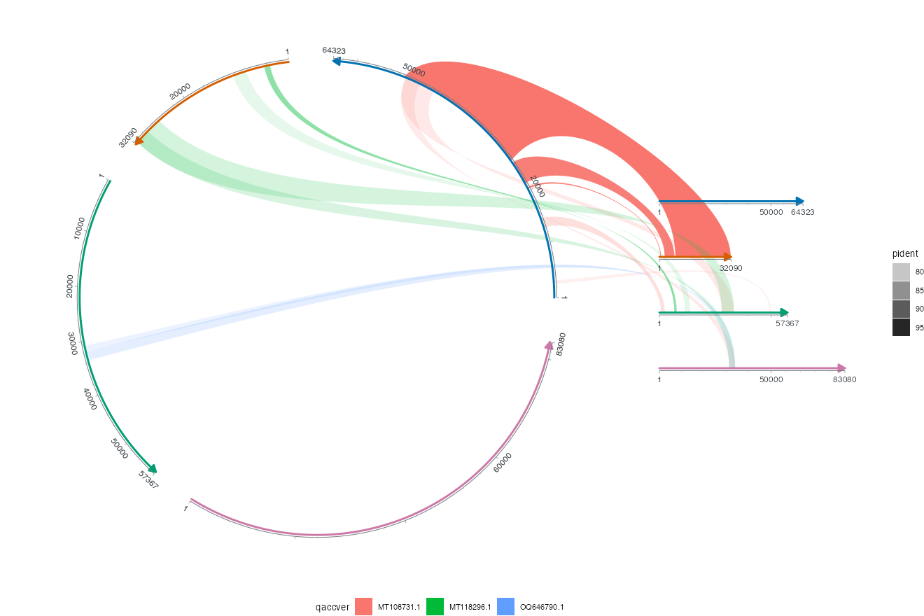
layout = "fixed" keeps existing placements. "adaptive" reuses the native Guide candidate/measurement engine, jointly considers side budgets and panel allocations, and then rebuilds every child in the remaining physical space. It may move/reflow unlocked Guides; explicit position, direction, rows/columns, fonts, key dimensions and absolute panel boxes remain constraints. For example, a default Identity ruler can become horizontal on a wide, short canvas; its length is remeasured for all six original labels rather than dropping 95 or 100.
metadata$guide_layout reports choices and locks. guide_bounds_mm and guide_sizes_mm describe the final outer boxes, after packaging and before panel measurement. Nested composition Guide reports appear in diagnostics. Impossible constraints fail explicitly. theme(legend.position = "none") hides composition Guides using native ggplot2 semantics. Inside composition Guides remain unsupported; each independent panel can still own local Guides. This is a bounded physical-space search, not a claim of global optimality.
4 Automatic perimeter panels
Set fusion_panel(..., side = "auto") to place more than eight independent panels around the center. The placement uses actual mm after the outer Guide budget, clockwise in input order on rectangular canvases. Explicit sizes and all fixed named/angle/box allocations stay fixed. Unlocked default containers may adapt down to a 15 mm floor; this does not shrink fonts or guarantee that arbitrary text will fit. Use each child’s own label/physical-size policy.
R · Example code
# Optional dependency: dplyr. One real HSP is deliberately shown 12 times.
library(ggchord)
library(dplyr)
observed <- ribbon_data_example |> slice_head(n = 1) |>
mutate(source_hsp_id = 'explicit-one-HSP-twelve-views')
source_seqs <- seq_data_example |> select(accver, length)
target_seqs <- source_seqs |> filter(accver == observed$saccver)
center <- ggchord(source_seqs) + geom_seq(show.legend = FALSE) +
geom_seq_label(size = 2.7) +
coord_chord() + theme(ggchord.axis = element_blank())
auto_fusion <- ggchord_fusion(center, layout = 'adaptive')
for (i in seq_len(12)) {
id <- paste0('view-', i)
view <- ggchord(target_seqs) + geom_seq(show.legend = FALSE) +
coord_collinear(seq_axis = if (i %% 2) 'horizontal' else 'vertical') +
theme(ggchord.axis = element_blank()) + ggplot2::labs(title = paste(id, observed$saccver, sep = '\n'))
auto_fusion <- auto_fusion +
fusion_panel(view, id, side = 'auto') +
fusion_ribbon(observed, qpanel = 'center', spanel = id, allow_repeated = TRUE,
fill = '#548CA0', alpha = .2)
}
view_ggchord(auto_fusion, width = 14, height = 10, units = "in")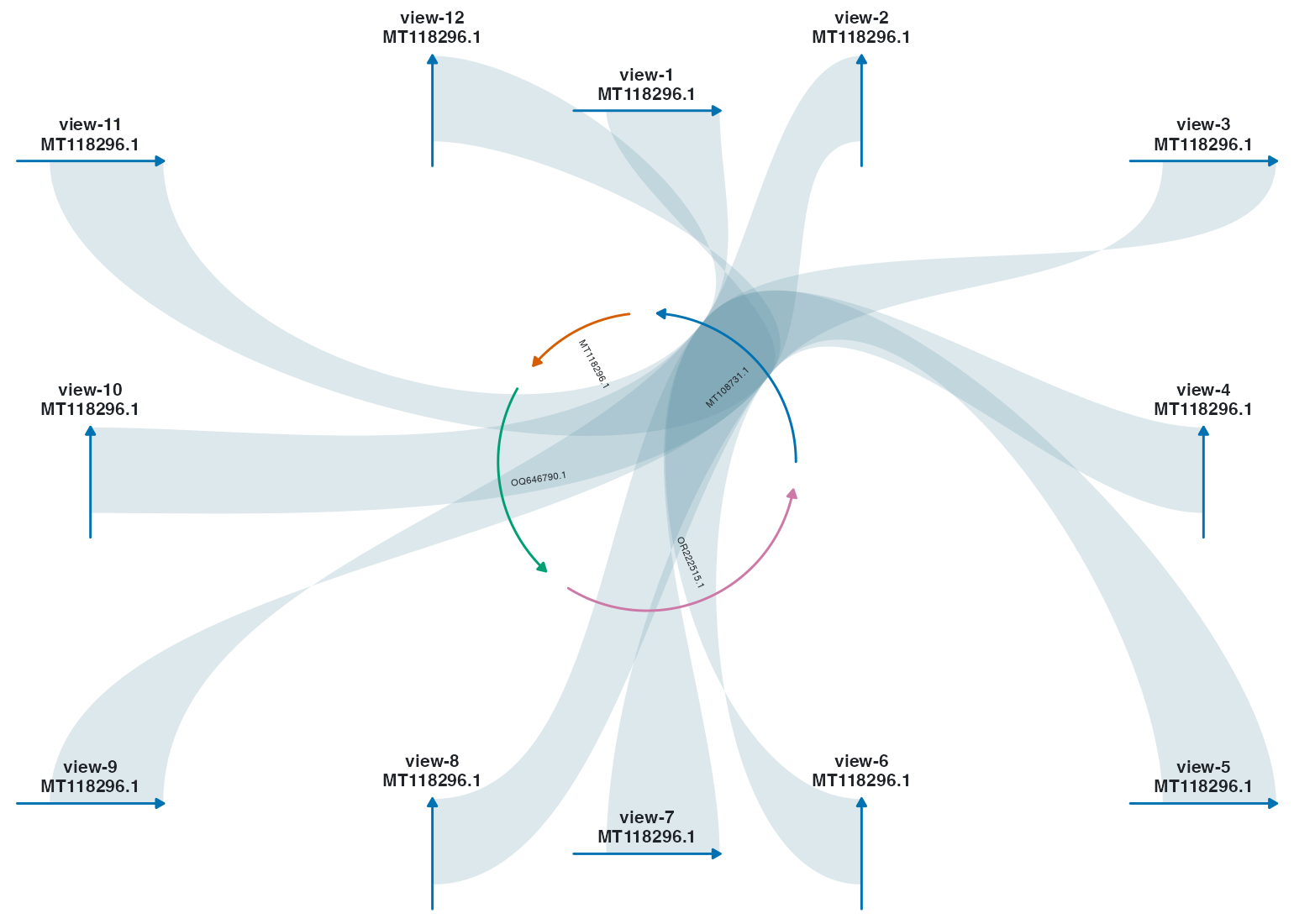
This real example intentionally displays one observed HSP twelve times. Its explicit source_hsp_id and allow_repeated = TRUE distinguish 12 connections from one observation. Each view still rebuilds its exact interval fronts. metadata$panel_layout records the bounded search, preserved constraints and container adaptation; panel rows expose auto_angle and auto_size_factor. Multiple magnify details can use repeated named "auto" sides, with explicit detail_panel selections. If no packing is feasible, the build fails with a clear diagnostic; no panel is discarded. The search is deterministic and conservative, not a global optimum or a promise that any count fits every canvas.
5 Native outer plot furniture
Use ordinary labs() and plot Theme elements for the composition’s title, subtitle, caption, tag, background and margins. These settings previously entered the style carrier without being drawn; they now reserve measured space and appear in the final static drawing. Each child retains its own axes, theme and source coordinates. Fusion has no Cartesian data axes.
R · Example code
styled_guide_fusion <- guide_fusion +
  ggplot2::labs(
    title = "Source-aware composition",
    subtitle = "Independent genomic panels and native Guides",
    caption = "Source: bundled ggchord records",
    tag = "A"
  ) +
  theme(
    plot.title = element_text(size = 16, face = "bold"),
    plot.caption = element_text(size = 9),
    plot.margin = margin(5, 5, 5, 5, "mm"),
    plot.background = element_rect(fill = "#F3F5F7", colour = NA)
  )
view_ggchord(styled_guide_fusion, width = 12, height = 8, units = "in")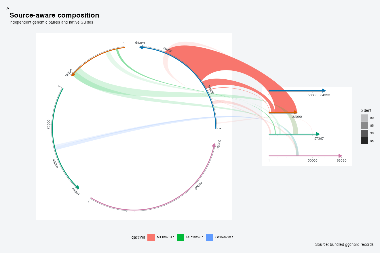
metadata$content_bounds_mm/content_canvas_mm describe the actual inner composition frame; plot_decoration records effective labels and native physical envelopes. Boxes refer to this content frame after outer decoration and Guide allocation. Existing fixed boxes are rechecked at target size; enlarge the canvas or revise explicit margins if they no longer fit. Clear headings with native labs(title = NULL, subtitle = NULL, caption = NULL, tag = NULL). No decoration keeps the previous rendering path.
Nested compositions retain independent headings and mm registration. Native foreground/background separation and inherited clipping keep translucent connections from accumulating repeated paints in explicit overlap mode. The source tables, selected intervals and palette mappings remain unchanged.
Ordinary child margins do not act as masks for composition connections. In explicit overlap mode, links traverse the full container below its foreground; later containers retain the declared covering order. Use measured route = "avoid" for annotation clearance instead of relying on accidental margin gaps.
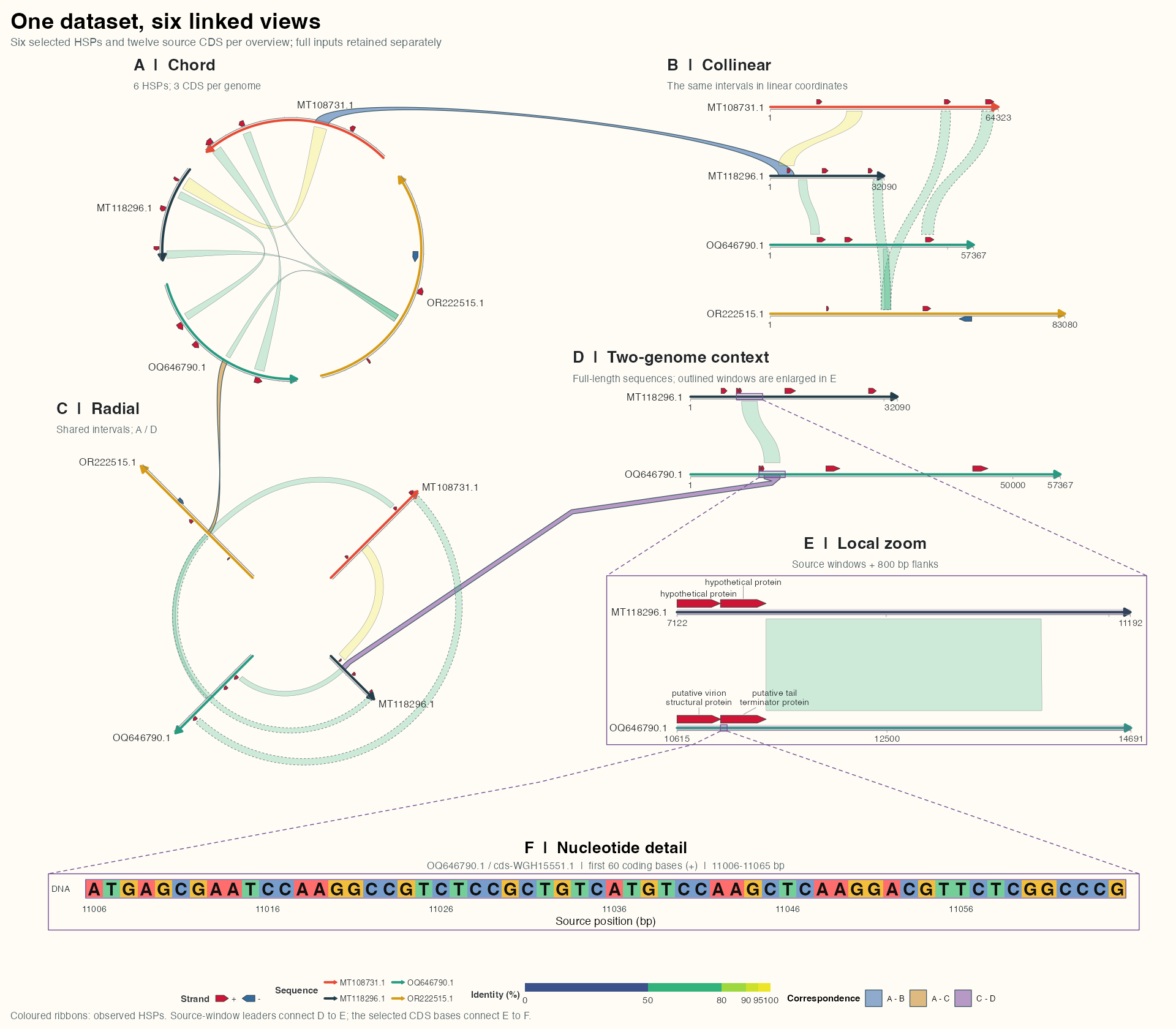
6 Integrated composition: global views and a local detail
Four independently valid views retain common sources. box controls physical allocation; focus_ggchord_data() explicitly prepares local windows. Cross-panel ribbons reuse source HSPs, and every participating layer declares repeated display.
R · Example code
library(ggchord)
library(ggplot2)
library(dplyr)
flagship_paper <- "#FFFCF5"
flagship_sequences <- flagship_dotplot_example$seq_data
flagship_hsp <- flagship_dotplot_example$links
flagship_features <- flagship_fusion_example$all_features
flagship_events <- flagship_fusion_example$events
flagship_colours <- c(
  "MT108731.1" = "#E64B35", "MT118296.1" = "#233E4A",
  "OQ646790.1" = "#269B82", "OR222515.1" = "#D59B17"
)
flagship_theme <- theme_ggchord_publication() +
  theme(
    plot.background = element_rect(fill = flagship_paper, colour = NA),
    panel.background = element_rect(fill = flagship_paper, colour = NA),
    legend.background = element_rect(fill = flagship_paper, colour = NA),
    legend.key = element_rect(fill = flagship_paper, colour = NA),
    legend.position = "right", legend.box = "vertical", legend.text = element_text(size = 8),
    legend.title = element_text(size = 9),
    plot.margin = margin(12, 16, 12, 16)
  )

flagship_position <- position_strand(0.045)
fusion_data <- flagship_fusion_example
fusion_orientation <- fusion_data$orientation
fusion_display_hsp <- fusion_data$links
fusion_display_features <- fusion_data$features
fusion_relation_ab <- fusion_data$relation_ab
fusion_relation_ac <- fusion_data$relation_ac
flagship_selected <- fusion_data$selected
flagship_windows <- fusion_data$windows
flagship_focused <- fusion_data$focused
fusion_detail_features <- fusion_data$detail_features
fusion_strand_colours <- c("+" = "#CE1536", "-" = "#346B9D")
fusion_shared_styles <- list(
  scale_seq_colour_manual(values = flagship_colours, limits = names(flagship_colours), drop = FALSE, name = "Sequence"),
  scale_gene_fill_manual(values = fusion_strand_colours, limits = c("+", "-"), drop = FALSE, name = "Strand"),
  guides(seq_colour = guide_ggchord_legend(nrow = 2, position = "bottom"),
    gene_fill = guide_ggchord_legend(nrow = 1, position = "bottom", override.aes = list(strand = c("+", "-"))),
    ribbon_fill = ggplot2::guide_coloursteps(available_aes = "ribbon_fill", even.steps = FALSE,
      show.limits = TRUE, position = "bottom", direction = "horizontal",
      theme = theme(legend.key.width = grid::unit(85, "mm"), legend.key.height = grid::unit(3, "mm")))),
  flagship_theme + theme(legend.position = "bottom", legend.box = "horizontal",
    legend.title = element_text(size = 9, face = "bold"), legend.text = element_text(size = 8),
    legend.margin = margin(2, 2, 2, 2), legend.spacing.x = grid::unit(2, "mm"),
    plot.margin = margin(3, 5, 3, 5), plot.title = element_text(size = 15, face = "bold", hjust = 0),
    plot.subtitle = element_text(size = 9, colour = "#52646A"),
    plot.title.position = "plot", ggchord.axis.text = element_text(size = 9))
)
make_fusion_view <- function(coord, title, subtitle, label_radius = NULL) {
  label_layer <- if (is.null(label_radius)) {
    geom_seq_label(size = 3.5, seq_label_orientation = "horizontal")
  } else {
    geom_seq_label(size = 3.5, seq_label_radius = label_radius,
      seq_label_orientation = "horizontal")
  }
  ggchord(flagship_sequences, fusion_display_hsp, feature_data = fusion_display_features) +
    geom_link_ribbon(adjacent_only = FALSE, alpha = 0.25, linewidth = 0.10,
      nonadjacent_linewidth = 0.22, allow_repeated = TRUE) +
    geom_seq(aes(seq_colour = accver), seq_orientation = fusion_orientation, linewidth = 1.1) +
    geom_gene(aes(gene_fill = strand), position = flagship_position, width = 0.04) +
    label_layer +
    coord + fusion_shared_styles + labs(title = title, subtitle = subtitle)
}
fusion_chord_view <- make_fusion_view(coord_chord(rotation = 45,
    xlim = c(-1.22, 1.02), ylim = c(-1.02, 1.22), fit = "manual"),
  "A  |  Chord", "6 HSPs; 3 CDS per genome", label_radius = 1.12) +
  theme(ggchord.axis.text = element_blank(), ggchord.axis.ticks = element_blank())
fusion_linear_view <- make_fusion_view(coord_collinear(ratio = 0.78),
  "B  |  Collinear", "The same intervals in linear coordinates") +
  scale_seq_position_continuous(n.breaks = 2, minor_breaks = NULL)
fusion_radial_view <- make_fusion_view(coord_radial_synteny(start_angle = 45, inner_radius = 0.7),
  "C  |  Radial", "Shared intervals; A / D") +
  theme(ggchord.axis.text = element_blank(), ggchord.axis.ticks = element_blank())
fusion_zoom_view <- ggchord(flagship_focused$seq_data, flagship_focused$ribbon_data,
  feature_data = fusion_detail_features) +
  geom_link_ribbon(allow_repeated = TRUE, alpha = 0.25, linewidth = 0.10) +
  geom_seq(aes(seq_colour = accver), seq_orientation = 1, linewidth = 1.1) +
  geom_gene(aes(gene_fill = strand), position = flagship_position, width = 0.04) +
  geom_gene_label_repel(size = 3.05, label_wrap = 22, label_max_lines = 2, position = flagship_position) +
  geom_seq_label(size = 3.5, seq_label_orientation = "horizontal") +
  coord_collinear(ratio = 0.85, fit = "manual",
    xlim = c(-0.42, 2.08), ylim = c(-0.72, 0.22)) + fusion_shared_styles +
  scale_seq_position_continuous(n.breaks = 3, minor_breaks = NULL, coordinates = "source") +
  labs(title = "E  |  Local zoom", subtitle = "Source windows + 800 bp flanks") +
  theme(plot.title = element_text(hjust = 0.5), plot.subtitle = element_text(hjust = 0.5))
fusion_context_sequences <- fusion_data$context_sequences
fusion_base_cds <- fusion_data$base_cds
fusion_base_start <- fusion_data$base_start
fusion_base_end <- fusion_data$base_end
fusion_base_cells <- fusion_data$base_cells
fusion_base_view <- ggplot(fusion_base_cells, aes(alignment_column, accver, label = symbol)) +
  geom_residue(overflow = "error", show.legend = FALSE) +
  scale_x_continuous(breaks = seq(1, 60, 10),
    labels = function(x) fusion_base_cells$source_position[match(x, fusion_base_cells$alignment_column)],
    expand = expansion(add = 0.6)) +
  scale_y_discrete(labels = setNames("DNA", fusion_base_cds$feature_id), expand = expansion(add = 0.7)) +
  labs(title = "F  |  Nucleotide detail", x = "Source position (bp)", y = NULL,
    subtitle = paste0(fusion_base_cds$accver, " / ", fusion_base_cds$feature_id,
      "  |  first 60 coding bases (", fusion_base_cds$strand, ")  |  ",
      fusion_base_start, "-", fusion_base_end, " bp")) +
  theme_minimal(base_size = 11) +
  theme(panel.grid = element_blank(), plot.background = element_rect(fill = flagship_paper, colour = NA),
    axis.text = element_text(colour = "#25363B"),
    plot.title = element_text(size = 16, face = "bold", hjust = 0.5),
    plot.subtitle = element_text(size = 10, colour = "#52646A", hjust = 0.5), plot.margin = margin(4, 12, 4, 12))
fusion_base_view <- register_ggchord_alignment(fusion_base_view, fusion_base_cells)
fusion_focus_regions <- fusion_data$focus_regions
fusion_context_features <- fusion_data$context_features
fusion_detail_view <- ggchord(fusion_context_sequences, flagship_selected, feature_data = fusion_context_features) +
  geom_link_ribbon(allow_repeated = TRUE, alpha = 0.25, linewidth = 0.10) +
  geom_seq(aes(seq_colour = accver), seq_orientation = 1, linewidth = 1.1) +
  geom_gene(aes(gene_fill = strand), position = flagship_position, width = 0.04) +
  geom_seq_label(size = 3.5, seq_label_orientation = "horizontal") +
  coord_collinear(ratio = 0.7) + fusion_shared_styles +
  scale_seq_position_continuous(n.breaks = 2, minor_breaks = NULL) +
  labs(title = "D  |  Two-genome context", subtitle = "Full-length sequences; outlined windows are enlarged in E")
flagship_detail <- fusion_zoom_view
fusion_connections <- list(
  fusion_ribbon(fusion_data$relation_ab, aes(fill = relation),
    qpanel = "chord", spanel = "linear", alpha = 0.65, colour = "#3E5763", linewidth = 0.35,
    curvature = 0.09, allow_repeated = TRUE),
  fusion_ribbon(fusion_data$relation_ac, aes(fill = relation),
    qpanel = "chord", spanel = "radial", alpha = 0.65, colour = "#3E5763", linewidth = 0.35,
    curvature = 0.2, allow_repeated = TRUE),
  fusion_ribbon(fusion_data$relation_cd, aes(fill = relation),
    qpanel = "radial", spanel = "center", alpha = 0.65, colour = "#3E5763", linewidth = 0.35,
    curvature = 0.2, route = "avoid", route_width = 1.5, allow_repeated = TRUE)
)
make_flagship_fusion <- function(preview = FALSE) {
  output_styles <- list(
    guides(ribbon_fill = ggplot2::guide_coloursteps(available_aes = "ribbon_fill",
      even.steps = FALSE, show.limits = TRUE, position = "bottom", direction = "horizontal",
      theme = theme(legend.key.width = grid::unit(if (preview) 90 else 85, "mm"),
        legend.key.height = grid::unit(3, "mm")))),
    theme(plot.title = element_text(size = if (preview) 15 else 16),
      plot.subtitle = element_text(size = if (preview) 9 else 10),
      legend.text = element_text(size = if (preview) 8 else 9))
  )
  lift <- function(box) c(box[1:2], 0.20 + 0.80 * box[3:4])
  out <- magnify_ggchord(fusion_detail_view + output_styles, region = fusion_focus_regions,
    detail_plot = list(zoom = fusion_zoom_view + output_styles, bases = fusion_base_view), guides = "collect",
    center_box = lift(c(0.465, 0.97, 0.385, 0.59)),
    detail_box = list(zoom = lift(c(0.49, 0.99, 0.01, 0.36)), bases = c(0.025, 0.985, 0, 0.17)),
    colour = "#725094", alpha = 0.20, highlight_width = 2.2,
    linewidth = 0.40, connector = "envelope", route = "avoid") +
    fusion_panel(fusion_chord_view + output_styles, id = "chord",
      box = lift(c(0.01, 0.455, if (preview) 0.52 else 0.54, 0.99))) +
    fusion_panel(fusion_linear_view + output_styles, id = "linear", box = lift(c(0.52, 0.995, 0.60, 0.99))) +
    fusion_panel(fusion_radial_view + output_styles, id = "radial",
      box = lift(c(0.01, 0.455, 0, if (preview) 0.50 else 0.52)))
  for (connection in fusion_connections) out <- out + connection
  out <- out + scale_fill_manual(name = if (preview) "Links" else "Correspondence", values = c("A - B" = "#527FB8",
    "A - C" = "#CE9741", "C - D" = "#9064AC")) +
    guides(fill = guide_legend(nrow = 1, position = "bottom",
      theme = if(preview) theme(legend.key.width = grid::unit(3, "mm"),
        legend.key.height = grid::unit(3, "mm")) else NULL)) +
    theme(plot.background = element_rect(fill = flagship_paper, colour = NA),
      legend.position = "bottom", legend.title = element_text(size = 9, face = "bold"),
      legend.text = element_text(size = 8), plot.title = element_text(size = 22, face = "bold", hjust = 0),
      plot.subtitle = element_text(size = 11, colour = "#52646A"),
      plot.caption = element_text(size = 10, colour = "#52646A", hjust = 0),
      plot.margin = margin(8, 10, 8, 10))
  if (!preview) out <- out + labs(title = "One dataset, six linked views",
    subtitle = "Six selected HSPs and twelve source CDS per overview; full inputs retained separately",
    caption = "Coloured ribbons: observed HSPs. Source-window leaders connect D to E; the selected CDS bases connect E to F.")
  out
}
flag_fusion <- make_flagship_fusion()