章节与参考
通用技巧 · 第 6 节,共 10 节
5.5 标度、图例与主题
本页目录
先确定数据含义,再选角色和标度。这里把同一批真实 HSP、注释与 GC 窗口分别用于连续值、类别、identity、透明度、线宽、线型与主题;无需为每个辅助函数创建一页。
1 独立输入与标度职责
本页独立加载 ggchord 和可选 dplyr。四条完整序列、HSP identity 与 query/subject ID 来自随包真实记录。命名向量用于把已有类别对应到显示值,不创造新的样本或统计量。映射写 aes,固定样式写 geom,用户 scale 优先于自动默认。显式固定属性会覆盖对应映射,想映射透明度时不要再传固定 alpha。
R · 示例代码
library(ggchord)
library(dplyr)
scale_seqs <- seq_data_example[c("accver", "length")]
scale_links <- ribbon_data_example
scale_ids <- scale_seqs$accver
scale_colours <- setNames(c("#E64B35", "#233E4A", "#269B82", "#D59B17"), scale_ids)
scale_opacity <- setNames(c(0.35, 0.55, 0.75, 0.95), scale_ids)
scale_lines <- setNames(c("solid", "dashed", "dotted", "dotdash"), scale_ids)
scale_base <- ggchord(scale_seqs, ribbon_data = scale_links) + geom_seq() + coord_chord()
scale_numeric <- scale_base + geom_link_ribbon(aes(ribbon_fill = pident))
2 连续、分段与直接颜色值
两图都将真实 pident 映射到 ribbon_fill,范围固定 0–100、配色和尺寸固定。gradientn 连续插值;stepsn 按给定 breaks 分段。颜色相同不证明新的同源关系。values 是渐变中的颜色锚点,不是原始 pident;breaks 控制刻度/分段,limits 控制数据域。NA 与越界值应检查标度策略,不当作零。
R · 示例代码
p_comparescalegradient <- scale_numeric +
  scale_ribbon_fill_gradientn(colours = c("#303B71", "#269B82", "#ECEB31"),
    limits = c(0, 100), breaks = c(0, 50, 80, 90, 95, 100), name = "Identity (%)") +
  guides(ribbon_fill = guide_ggchord_colourbar())
view_ggchord(p_comparescalegradient, width = 9, height = 7, units = "in")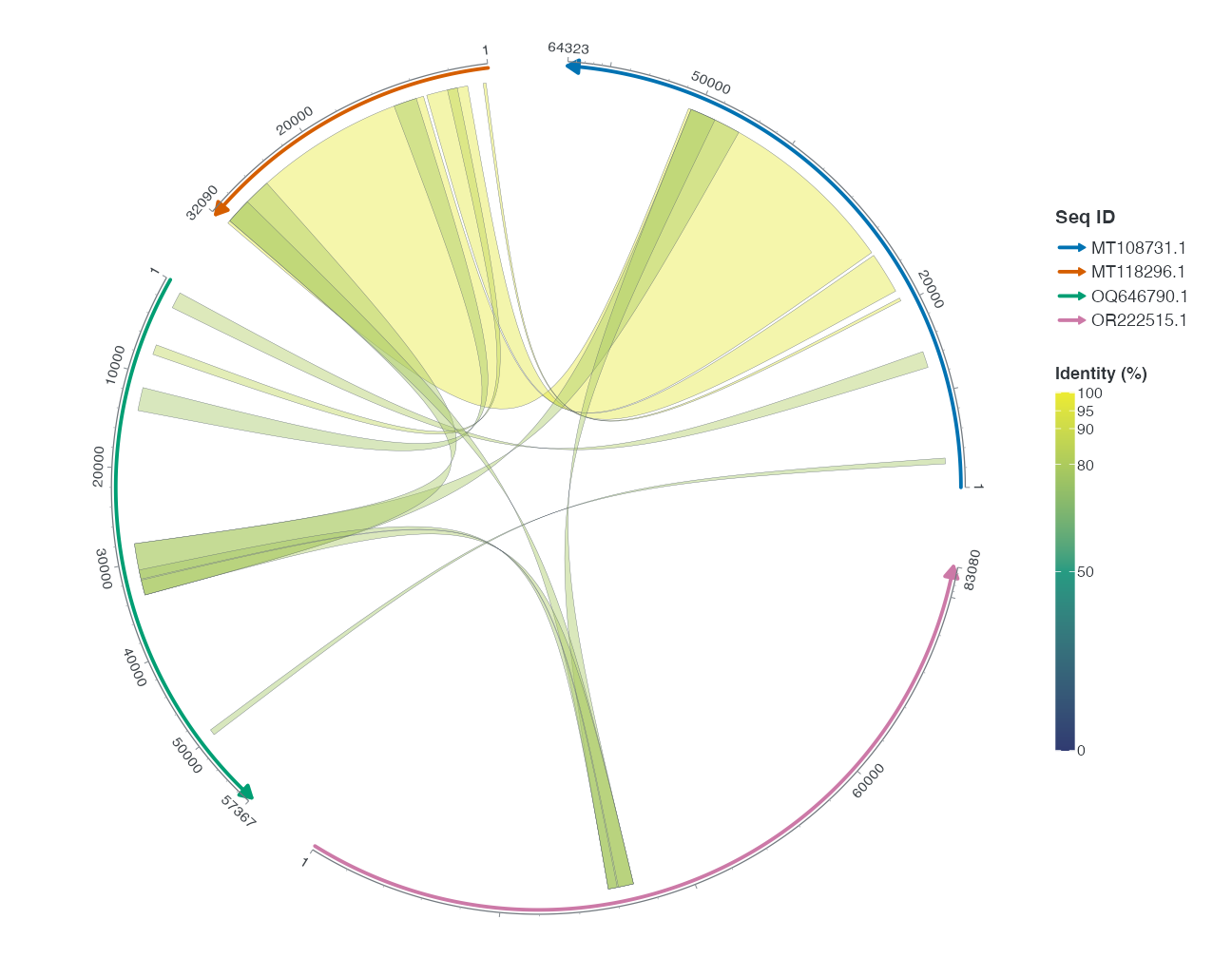
R · 示例代码
p_comparescalesteps <- scale_numeric +
  scale_ribbon_fill_stepsn(colours = c("#303B71", "#269B82", "#ECEB31"),
    breaks = c(0, 50, 80, 90, 95, 100), limits = c(0, 100),
    name = "Identity (%)", guide = ggplot2::guide_coloursteps(available_aes = "ribbon_fill",
      even.steps = FALSE, show.limits = TRUE, position = "left",
      direction = "vertical", theme = theme(legend.key.height = grid::unit(80, "mm"))))
view_ggchord(p_comparescalesteps, width = 9, height = 7, units = "in")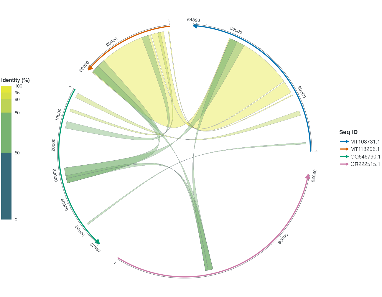
3 identity 不再替数据选色
下面先从真实 identity 按显式 90% 阈值生成显示颜色,再用 scale_ribbon_fill_identity 直接读取颜色字符串。这是事先声明的显示分类,不是恢复连续 identity 的方法。若需要连续图例,用上一节的渐变。identity 通常不显示图例;要显示时必须明确 breaks、labels 和 guide,使图例解释颜色的业务含义。
R · 示例代码
scale_identity_links <- scale_links |>
  mutate(display_colour = if_else(pident >= 90, "#269B82", "#303B71"))
p_scale_identity <- ggchord(scale_seqs, ribbon_data = scale_identity_links) +
  geom_seq() + geom_link_ribbon(aes(ribbon_fill = display_colour)) +
  scale_ribbon_fill_identity() + coord_chord()
invisible(ggplot2::ggplot_build(p_scale_identity))
4 类别填色、透明度、边框与线型
同一 qaccver 映射到同一显示值。manual 系列的 values 推荐按实际类别命名,避免类别顺序变化后错配。此例同时训练多个独立角色,是组合示范,不是单参数视觉对照。连续透明度用 scale_ribbon_alpha_continuous(range=...);离散透明度用 scale_ribbon_alpha_manual。colour 与 linetype 只改变边框;不能用边框外观代替区间方向。
R · 示例代码
p_scale_manual <- scale_base +
  geom_link_ribbon(aes(ribbon_fill = qaccver, ribbon_alpha = qaccver,
    ribbon_colour = qaccver, ribbon_linetype = qaccver)) +
  scale_ribbon_fill_manual(values = scale_colours) +
  scale_ribbon_alpha_manual(values = scale_opacity) +
  scale_ribbon_colour_manual(values = scale_colours) +
  scale_ribbon_linetype_manual(values = scale_lines) +
  scale_seq_colour_manual(values = scale_colours) +
  guides(ribbon_fill = guide_ggchord_legend(nrow = 1))
invisible(ggplot2::ggplot_build(p_scale_manual))
5 点连接的独立标度家族
先从真实 HSP 显式计算中点;不把点连接当作覆盖整个比对区间。manual 系列分别给 link_colour、link_alpha、link_linewidth、link_linetype 映射类别;gradientn、alpha_continuous、linewidth_continuous 对应数值。下面先构造类别组合,再用 pident 训练连续组合。
自动托管的数值 pident 映射使用0–100域和0、50、80、90、95、100六个Identity刻度;显式用户标度继续优先。此例为三个通道设置相同域、刻度与标题,使图例键可以合并。
R · 示例代码
scale_points <- scale_links |>
  slice_head(n = 6) |>
  mutate(qpos = floor((qstart + qend) / 2), spos = floor((sstart + send) / 2))
p_scale_linkbase <- ggchord(scale_seqs) + geom_seq() + coord_chord()
R · 示例代码
p_scale_linkmanual <- p_scale_linkbase +
  geom_link_line(aes(link_colour = saccver, link_alpha = saccver,
    link_linewidth = saccver, link_linetype = saccver), data = scale_points) +
  scale_link_colour_manual(values = scale_colours) +
  scale_link_alpha_manual(values = scale_opacity) +
  scale_link_linewidth_manual(values = setNames(c(0.3, 0.5, 0.7, 0.9), scale_ids)) +
  scale_link_linetype_manual(values = scale_lines)
invisible(ggplot2::ggplot_build(p_scale_linkmanual))
R · 示例代码
p_comparescalelinkcontinuous <- p_scale_linkbase +
  geom_link_line(aes(link_colour = pident, link_alpha = pident,
    link_linewidth = pident), data = scale_points) +
  scale_link_colour_gradientn(
    colours = c("#303B71", "#ECEB31"), limits = c(0, 100),
    breaks = c(0, 50, 80, 90, 95, 100), name = "Identity (%)",
    guide = guide_ggchord_legend()
  ) +
  scale_link_alpha_continuous(
    range = c(0.3, 0.9), limits = c(0, 100),
    breaks = c(0, 50, 80, 90, 95, 100), name = "Identity (%)"
  ) +
  scale_link_linewidth_continuous(
    range = c(0.2, 1), limits = c(0, 100),
    breaks = c(0, 50, 80, 90, 95, 100), name = "Identity (%)"
  )
view_ggchord(p_comparescalelinkcontinuous, width = 9, height = 7, units = "in")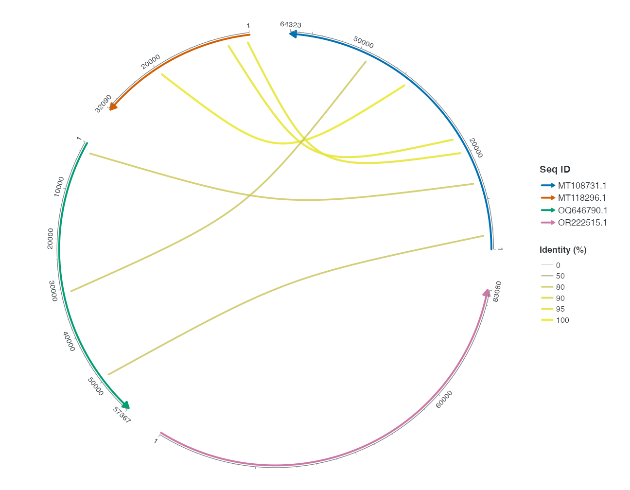
6 注释、基因与区域角色
feature_fill 和 feature_shape 可按同一个 type 映射,形状与填色图例可合并;独立 shape guide 需要显式请求。固定 shape 会优先于形状映射。这里所有 type 先用 arrow,是为了演示映射规则而不赋予未验证的形状功能。质粒 fill/shape 预设使用其记录的类别规则。
R · 示例代码
scale_feature_data <- head(find_common_features(plasmid_example_pUC19), 6)
feature_types <- unique(scale_feature_data$type)
feature_colours <- setNames(rep(c("#993366", "#31849B", "#D59B17"),
  length.out = length(feature_types)), feature_types)
p_scale_feature <- ggchord(plasmid_example_pUC19) + geom_seq() +
  geom_feature(aes(feature_fill = type, feature_shape = type), data = scale_feature_data) +
  scale_feature_fill_manual(values = feature_colours) +
  scale_feature_shape_manual(values = setNames(rep("arrow", length(feature_types)), feature_types)) +
  coord_circular()
invisible(ggplot2::ggplot_build(p_scale_feature))
R · 示例代码
p_scale_preset <- ggchord(plasmid_example_pUC19) + geom_seq() +
  geom_feature(aes(feature_fill = type, feature_shape = type), data = scale_feature_data) +
  scale_feature_fill_plasmid() + scale_feature_shape_plasmid() + coord_circular()
invisible(ggplot2::ggplot_build(p_scale_preset))
7 基因链、序列 ring 与局部区域
基因链采用原始 source_strand。region_fill 与 gene_fill、ribbon_fill 互不覆盖。seq_ring 必须有显式正半径表,不推断轨道数量;不能再同时传 seq_radius,也不能用于共线性图。它是序列半径映射,不等于定量 position_track 的命名轨道。
R · 示例代码
scale_gene_data <- gene_data_example |>
  transmute(accver, start, end, strand = source_strand)
p_scale_gene <- ggchord(scale_seqs, gene_data = scale_gene_data) + geom_seq() +
  geom_gene() + scale_gene_fill_manual(values = c("+" = "#CE1536", "-" = "#346B9D")) + coord_chord()
p_scale_ring <- ggchord(scale_seqs) + geom_seq(aes(seq_ring = accver)) +
  scale_seq_ring_manual(values = setNames(c(0.8, 1, 1.2, 1.4), scale_ids)) + coord_chord()
invisible(ggplot2::ggplot_build(p_scale_gene))
invisible(ggplot2::ggplot_build(p_scale_ring))
R · 示例代码
scale_region_data <- scale_links |>
  slice_head(n = 3) |>
  transmute(accver = qaccver, start = pmin(qstart, qend), end = pmax(qstart, qend))
p_scale_region <- ggchord(scale_seqs) + geom_seq() +
  geom_seq_region(aes(region_fill = accver), data = scale_region_data) +
  scale_region_fill_manual(values = scale_colours) + coord_chord()
invisible(ggplot2::ggplot_build(p_scale_region))
8 命名轨道的值域与颜色
先用真实 pUC19 DNA 计算窗口。track_value 控制数值高度,track_fill/track_colour 训练各自颜色;track ID 必须和 position_track 一致。下面的分类阈值 0.5 是显示选择,完整比例值仍保留。tile 不自动求均值,不把 NA 高度变成零。多个 ID 的颜色和数值标度分别声明。
R · 示例代码
plasmid <- plasmid_example_pUC19
track_seq <- plasmid[c("accver", "length")]
starts <- seq.int(1, plasmid$length, by = 100)
bins <- data.frame(accver = plasmid$accver, start = starts,
                   end = pmin(starts + 99, plasmid$length))
bins$gc <- vapply(seq_len(nrow(bins)), function(i) {
  bases <- strsplit(substr(plasmid$sequence, bins$start[i], bins$end[i]), "")[[1]]
  mean(bases %in% c("G", "C"))
}, numeric(1))
head(bins)
R · 示例代码
scale_track_bins <- bins |>
  mutate(gc_class = if_else(gc >= 0.5, "GC >= 0.5", "GC < 0.5"))
p_scale_trackfill <- ggchord(track_seq) + geom_seq() +
  geom_track_tile(aes(track_fill = gc_class), data = scale_track_bins,
    position = position_track("classes")) +
  scale_track_fill_manual("classes", values = c("GC >= 0.5" = "#31849B", "GC < 0.5" = "#D59B17")) +
  coord_circular()
p_scale_trackcolour <- ggchord(track_seq) + geom_seq() +
  geom_track_tile(aes(track_colour = gc_class), data = scale_track_bins,
    position = position_track("classes"), fill = NA) +
  scale_track_colour_manual("classes", values = c("GC >= 0.5" = "#31849B", "GC < 0.5" = "#D59B17")) +
  coord_circular()
invisible(ggplot2::ggplot_build(p_scale_trackfill))
invisible(ggplot2::ggplot_build(p_scale_trackcolour))
R · 示例代码
p_scale_trackgradient <- ggchord(track_seq) + geom_seq() +
  geom_track_tile(aes(track_fill = gc, track_colour = gc), data = bins,
    position = position_track("gc")) +
  scale_track_fill_gradientn("gc", colours = c("#D59B17", "#31849B")) +
  scale_track_colour_gradientn("gc", colours = c("#D59B17", "#31849B")) +
  coord_circular()
invisible(ggplot2::ggplot_build(p_scale_trackgradient))
9 guide、别名与 staged mapping
guide_ggchord_legend 管理离散角色图例;guide_ggchord_colourbar 管理连续颜色条。show.legend 控制图层是否参与,guides 选择图例,theme 控制位置、方向与外观。colour/color 拼写别名有相同语义:guide_ggchord_colorbar、scale_seq_color_manual、scale_ribbon_color_manual、scale_link_color_manual、scale_link_color_gradientn 分别对应 colour 版本,不能同时添加两种同义标度来叠加控制。
after_stat 读取统计变量,例如下一课的 bundle_n;after_scale 在标度之后计算受支持的视觉属性。两者来自 ggplot2,即使 R 对象看起来相同,staged mapping 的语义也不同。所有 ggplot2/grid 重导出遵循其上游帮助,参数图谱明确区分归属。
10 主题只表达非数据外观
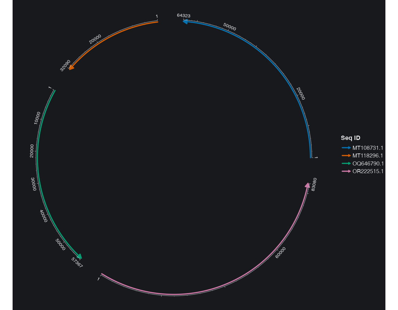
theme_ggchord、minimal、publication、dark 是共享非数据样式的不同起点;plasmid 适合单序列圆图。下面两个图只有主题不同,骨架与数据映射不变。theme 中的轴间距、刻度长、文字偏移使用文档声明的物理单位;自定义主题字段不是按 accver 命名的几何列表。只关闭文字会隐藏文字,不会删除序列。
R · 示例代码
theme_examples <- list(
  default = theme_ggchord(), minimal = theme_ggchord_minimal(),
  publication = theme_ggchord_publication(), dark = theme_ggchord_dark()
)
for (selected_theme in theme_examples) {
  invisible(ggplot2::ggplot_build(scale_base + selected_theme))
}
p_comparethememinimal <- scale_base + theme_ggchord_minimal()
p_comparethemedark <- scale_base + theme_ggchord_dark()
p_theme_plasmid <- ggchord(plasmid_example_pUC19) + geom_seq() +
  coord_circular() + theme_ggchord_plasmid()
invisible(ggplot2::ggplot_build(p_theme_plasmid))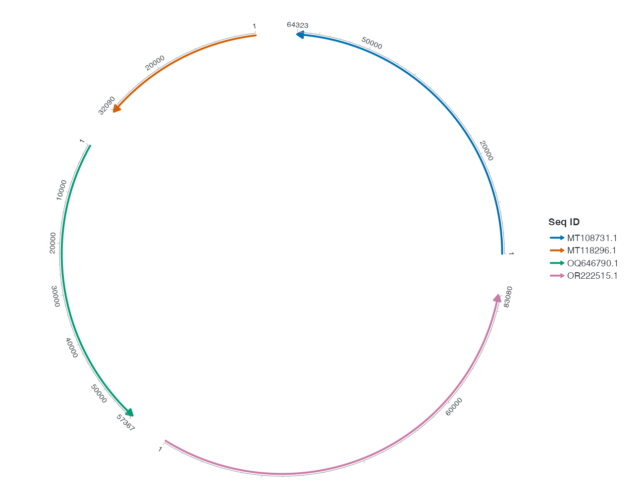
11 操作示例与选择规则
先把 pident 映射从连续渐变改为显式分段,再改回渐变,只改变 alpha 输出范围;核对图例是否仍表示相同数据单位。新增图层时给每层独立 data/mapping,保留已存在的用户 scale。完整参数、类型、默认与转发边界见参数图谱;聚束和密度见连接统计。