章节与参考
通用技巧 · 第 3 节,共 10 节
5.2 基因与特征的箭头几何
用同一个真实 CDS 比较箭头轮廓。先看形状,再选择尺寸;改变轮廓不会改变区间、链或生物学功能。
1 准备真实注释与局部窗口
示例来自随包 gene_data_example 的 integrase:OQ646790.1 的 43,765–46,140 bp。链从 source_strand 恢复为原始正链。窗口取 43,000–47,000 bp,只为放大观察,坐标轴显示源坐标。
R · 示例代码
library(ggchord)
library(dplyr)
source_gene <- gene_data_example |>
  filter(accver == "OQ646790.1", start == 43765) |>
  transmute(accver, start, end, strand = source_strand, anno)
gene_window <- focus_ggchord_data(
  seq_data = filter(seq_data_example, accver == "OQ646790.1"),
  gene_data = source_gene,
  loci = data.frame(accver = "OQ646790.1", start = 43000, end = 47000)
)
gene_base <- ggchord(gene_window$seq_data, gene_data = gene_window$gene_data) +
  geom_seq() +
  scale_seq_position_continuous(coordinates = "source") +
  coord_collinear()
gene_window 保留裁剪与来源元数据。换用自己的 CDS 时,需要完整序列长度、匹配的 accver、一基闭区间 start/end 和证据支持的正负链;未知链用 geom_feature()。本页可在新 R 会话独立运行,需安装可选依赖 dplyr。
2 用明确 ID 选出真实邻域
这里把来源 accession 与端点组合成工作流 target ID,不假称它是数据库基因 ID。find_ggchord_loci 按 ID 精确选取,再在生物学方向上下游各扩展 100 bp;负链上游向较大的源坐标扩展,未知/双向链需使用对称扩展。返回窗口可传给 focus_ggchord_data,截断标记说明是否触及完整序列边界。
输出 / 文本
               target_id               locus_id     accver start   end strand target_start target_end upstream downstream clipped_left clipped_right target_source_rows
1 OQ646790.1:43765:46140 OQ646790.1:43765:46140 OQ646790.1 43665 46240      +        43765      46140      100        100        FALSE         FALSE                  1
3 三种箭头构造
三图均为 9 × 4 英寸,使用相同输入、窗口和图层。为了看清肩部,三图共同显式设置 arrow_head_width = 1.6(默认 1),每次只改变 arrow_head_style。
R · 示例代码
p_comparegeneshouldered <- gene_base + geom_gene(arrow_head_width = 1.6, arrow_head_style = "shouldered")
view_ggchord(p_comparegeneshouldered, width = 9, height = 4, units = "in")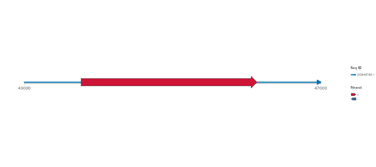
shouldered 是默认构造。头部较宽时,头身连接处有肩部,便于辨识箭头方向。
R · 示例代码
p_comparegeneflush <- gene_base + geom_gene(arrow_head_width = 1.6, arrow_head_style = "flush")
view_ggchord(p_comparegeneflush, width = 9, height = 4, units = "in")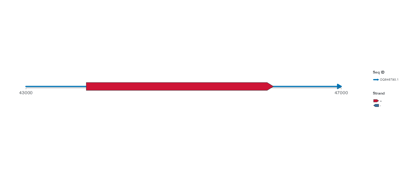
flush 用平齐的头身轮廓。对照同一端点和主体,看头部如何接入箭身。
R · 示例代码
p_comparegenetriangle <- gene_base + geom_gene(arrow_head_width = 1.6, arrow_head_style = "triangle")
view_ggchord(p_comparegenetriangle, width = 9, height = 4, units = "in")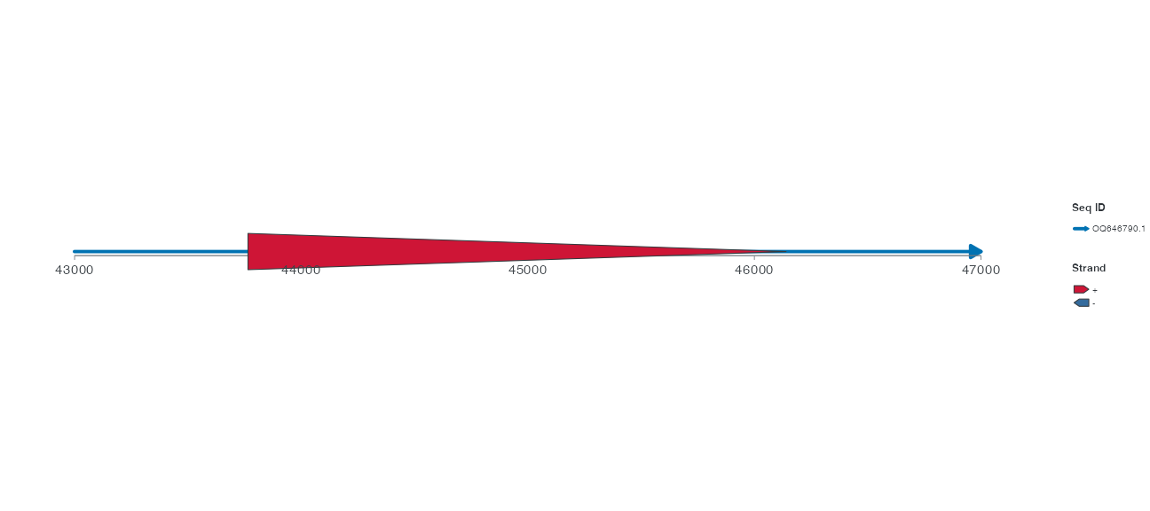
triangle 将整个区间画成三角楔形,而不是给长方形箭身加箭头。不能把形状区别解释为不同功能或测量值。
4 短特征放不下头部时
保留同一真实 integrase 与窗口,共同将请求头长设为 1.5,使区间相对请求头部变短。这里只改变 short_feature:auto 选择压缩的有向符号,wedge 使用楔形,block 使用无箭头的块。不要修改原始坐标把基因变长;无箭头显示也不表示源链未知。
R · 示例代码
p_compareshortauto <- gene_base + geom_gene(arrow_head_length = 1.5, short_feature = "auto")
view_ggchord(p_compareshortauto, width = 9, height = 4, units = "in")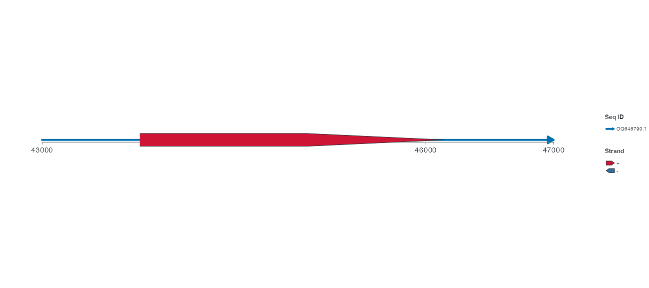
R · 示例代码
p_compareshortwedge <- gene_base + geom_gene(arrow_head_length = 1.5, short_feature = "wedge")
view_ggchord(p_compareshortwedge, width = 9, height = 4, units = "in")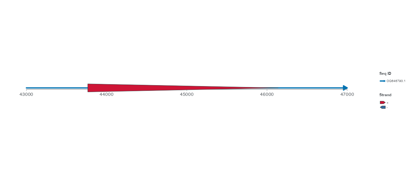
R · 示例代码
p_compareshortblock <- gene_base + geom_gene(arrow_head_length = 1.5, short_feature = "block")
view_ggchord(p_compareshortblock, width = 9, height = 4, units = "in")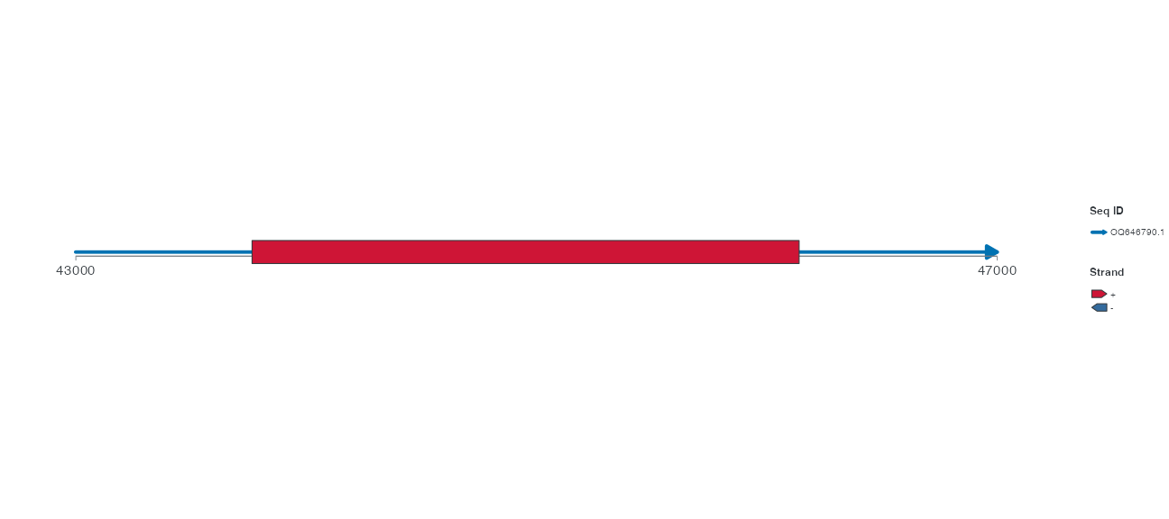
5 尺寸、短特征与预设
| 参数 |
geom_gene() 默认 |
取值与选择 |
|---|---|---|
width |
NULL,运行时为 0.05 |
箭身宽度;可按序列或链配置 |
arrow_head_length |
0.04 |
局部坐标中的头部长度;不按 bp 解释 |
arrow_head_width |
1 |
头部相对箭身的宽度;三图共同设为 1.6 |
arrow_head_style |
"shouldered" |
shouldered / flush / triangle |
short_feature |
"auto" |
放不下头部时选择 wedge 或 block;显式 wedge/block 固定回退策略 |
position |
"identity" |
按链分离用 position_strand;重叠分层用 position_feature_stack |
不要用放大头部长度掩盖短区间。先核查真实长度,再决定短特征策略。geom_feature() 的形状可用固定 shape 或 aes(feature_shape = ...) 与相应标度;固定和映射的职责见样式。
geom_feature_plasmid() 是具有不同默认宽度、头部尺寸和 Position 的预设。比较它与 gene 时若同时改变多个默认值,就不是单参数实验。分段注释的边界线用于标识分段,不表示不同基因。
6 模式、操作示例和下一步
基因箭头可用于弦图、共线性图和单序列圆图的 bp 数据;蛋白 aa 区间用通用特征。局部窗口与显示翻转不改写原始链,见兼容边界。
先只将共同头部宽度从 1.6 改回 1,比较肩部是否还明显;再仅改变 width,观察箭身与骨架的相对宽度。按相同设备尺寸比较,不调整源区间来改善外观。
相关功能特征堆叠、标签,或将同一 CDS 加入四基因组案例。完整接口见 geom_gene()、geom_feature()。