Chapters and reference
Module III · Sequence alignment Dotplot · Section 2 of 2
3.1 HSP axes, orientation and mapping
On this page
See Flagship data sources and construction for provenance, display selections and rebuilding. This page loads bundled inputs directly and focuses on plotting settings.
Start with observed HSPs from one sequence pair, then extend to a four-sequence matrix. The minimal inputs are complete sequence lengths and four HSP endpoints; annotations are optional.
1 Plot original HSP endpoints
Bundled sequence_detail_example$paf retains the 11 observed HSPs for the EMALE pair; sequence lengths declared by the source file define both axes. The table is already normalized to one-based coordinates; reverse-alignment target endpoints remain descending. Original files and provenance are available under input downloads. Preparation requires optional dplyr.
Each line runs from (qstart, sstart) to (qend, send). geom_seq() is not required. Use link_* mappings and scales for colour, alpha, width and type. The default Identity domain is 0–100 with ticks 0/50/80/90/95/100; an explicit user scale overrides it.
R · Example code
p_viewdotplot <- ggchord(dotplot_seqs, dotplot_hsp) +
geom_alignment_segment(aes(link_colour = pident), linewidth = 0.65) +
coord_dotplot()
view_ggchord(p_viewdotplot, width = 8, height = 7, units = "in")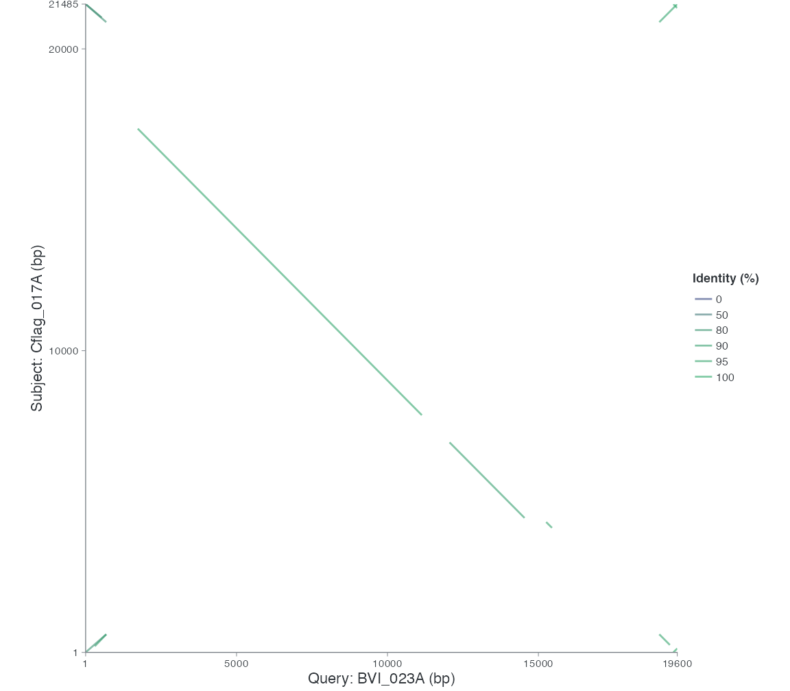
The legacy constructor may warn about descending endpoints in these valid reverse HSPs. Keep the normalized ordering; sorting each interval would erase the displayed inversion.
x_seqs and y_seqs independently select/order accessions. gap is display spacing in native bp/aa, not omitted source sequence. Axis directions accept 1/-1 or complete named vectors. Display reversal changes the slope without changing the biological source table. Each axis starts at source position 1; concatenated segments retain their own accession and local tick labels.
R · Example code
dotplot_reversed <- ggchord(dotplot_seqs, dotplot_hsp) +
geom_alignment_segment(aes(link_colour = pident), linewidth = 0.65) +
coord_dotplot(y_orientation = -1)
dotplot_layout <- export_ggchord_layout(dotplot_reversed)
dotplot_layout$axis_layoutUse map_ggchord_position(..., axis = "x"/"y") for native/global conversion, with inverse = TRUE to go back. Display gaps return NA. Focused source origins use source = TRUE; default axis labels stay window-relative. Unknown directions are warned, omitted and reported; contradictory direction metadata is rejected. Repeated declared HSP IDs require allow_repeated=TRUE in all participating layers. Unidentified duplicate/self rows remain distinct. Without cg/cs/CIGAR or another alignment trace, these are HSP segments, not base-level mismatches or gap paths.
2 Multi-sequence HSP matrix
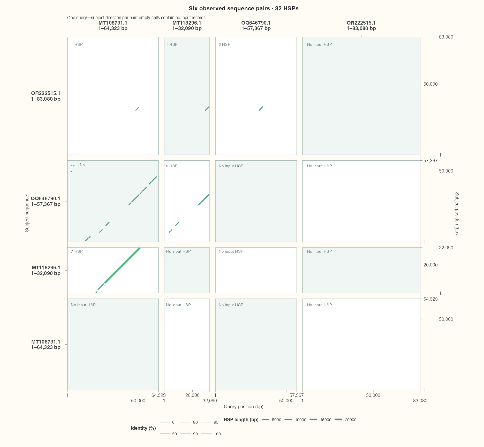
The following code directly uses bundled flagship_dotplot_example, with counts and label tables already prepared. It retains all 32 HSPs across four sequences without inventing self-alignments, symmetric records or missing HSPs. The 266 CDS belong to the shared source table but are not passed to the Dotplot segment layer. Empty regions indicate no relationship records in this input, not an absence of homology.
Column headers identify each query sequence and its complete 1–length range; row headers identify subject sequences and ranges. Bottom and right ticks show local positions within each sequence. Follow a column and row to locate a pair. Each outlined rectangle retains widths and heights proportional to the actual lengths. Pale backgrounds distinguish cells and do not encode similarity; spaces between rectangles are display gaps.
Each of the six unordered sequence pairs supplies only one query→subject direction, with no swapped records or self-alignments. HSPs therefore occupy one half of the matrix. Cells identify record counts or missing input. This is not a rendering omission, and an empty counterpart does not establish absent homology. The plot does not mirror records, add a diagonal or run new alignments. This preparation also uses optional tidyr.
Data preparation and settings (expand)
R · Example code
library(ggchord)
library(dplyr)
flagship_paper <- "#FFFCF5"
flagship_sequences <- flagship_dotplot_example$seq_data
flagship_hsp <- flagship_dotplot_example$links
flagship_theme <- theme_ggchord_publication() +
theme(
plot.background = element_rect(fill = flagship_paper, colour = NA),
panel.background = element_rect(fill = flagship_paper, colour = NA),
legend.background = element_rect(fill = flagship_paper, colour = NA),
legend.key = element_rect(fill = flagship_paper, colour = NA),
legend.position = "right", legend.box = "vertical", legend.text = element_text(size = 8),
legend.title = element_text(size = 9),
plot.margin = margin(12, 16, 12, 16)
)R · Example code
dotplot_pair_counts <- flagship_dotplot_example$pair_counts
dotplot_cells <- flagship_dotplot_example$cell_labels
flag_dotplot <- ggchord(flagship_sequences, flagship_hsp) +
  geom_alignment_segment(aes(link_colour = pident, link_linewidth = length), alpha = 0.85) +
  scale_link_linewidth_continuous(range = c(0.8, 1.8), name = "HSP length (bp)") +
  coord_dotplot(x_seqs = flagship_sequences$accver, y_seqs = flagship_sequences$accver,
    gap = 4000) +
  ggplot2::geom_text(data = dotplot_cells, aes(x = x, y = y, label = label),
    inherit.aes = FALSE, hjust = 0, vjust = 1, size = 2.8, colour = "#566E67") +
  labs(title = "Six observed sequence pairs · 32 HSPs",
    subtitle = "One query→subject direction per pair; empty cells contain no input records") +
  flagship_theme +
  theme(
    panel.grid = element_blank(), legend.position = "bottom", legend.box = "horizontal",
    axis.text = element_text(size = 9),
    axis.text.x.top = element_text(size = 10, face = "bold", margin = margin(b = 9)),
    axis.text.y.left = element_text(size = 10, face = "bold", margin = margin(r = 9)),
    axis.text.y.right = element_text(size = 9),
    axis.ticks.length = unit(1.5, "mm"),
    plot.margin = margin(12, 16, 12, 16)
  )
3 Inspect source direction
Relative endpoint direction comes from the source record. Reversing a display axis changes the visible slope while leaving the source direction unchanged. Count the supplied directions per sequence pair:
4 Query an exact position
Map the first HSP query start onto the concatenated x axis. Inverse lookup uses inverse = TRUE and an explicit axis; display gaps return NA. The four endpoints remain unchanged.
R · Example code
map_ggchord_position(
  flag_dotplot, flagship_hsp$qaccver[1], flagship_hsp$qstart[1], axis = "x"
)
5 Boundaries and next steps
Backbone gene/feature/track/ribbon layers, facets and Fusion endpoints are unsupported. To inspect gaps or mismatches, provide actual aligned characters; see the alignment workflow. Example: trace four endpoints of one segment and explain slope and colour separately.