ggchord tutorial

library(ggchord)
library(ggplot2)

data(seq_data_example)
data(ribbon_data_example)
data(gene_data_example)

This tutorial walks through the complete ggchord workflow: preparing input data, importing files in R, validating and cleaning data, and building plots layer by layer. It documents the v0.9.0 release.

1. Data preparation

Three types of input data are used. All three are plain data frames.

[Required] Sequence data (`seq_data`)

Column	Type	Description
`seq_id`	character	Unique sequence identifier
`length`	integer	Sequence length (must be positive)

Example:

seq_id	length
MT108731.1	64323
MT118296.1	32090
OQ646790.1	57367
OR222515.1	83080

A common way to build this table from FASTA files:

seqkit fx2tab -nil examples/fasta/*.fna | sed '1i seq_id\tlength' > examples/seq_track.tsv

[Optional] Alignment data (`ribbon_data`)

One row per alignment block between two sequences (the column names follow common alignment-tool conventions):

Column	Type	Description
`qaccver`	character	Query sequence ID
`saccver`	character	Subject sequence ID
`length`	integer	Alignment length (bp)
`pident`	numeric	Percent identity (0–100)
`qstart`	integer	Start position on the query sequence
`qend`	integer	End position on the query sequence
`sstart`	integer	Start position on the subject sequence
`send`	integer	End position on the subject sequence

Example rows:

qaccver	saccver	length	pident	qstart	qend	sstart	send
MT108731.1	MT118296.1	24856	98.612	26298	51139	7121	31959
MT108731.1	MT118296.1	4412	97.031	21513	25922	2365	6772
MT108731.1	MT118296.1	464	94.181	20691	21146	1032	1495

For example, the standard BLAST -outfmt 7 output can be parsed into this table directly:

seqs=("MT108731.1" "MT118296.1" "OQ646790.1" "OR222515.1")
ext="fna"
for ((i=0; i<${#seqs[@]}-1; i++)); do
  for ((j=i+1; j<${#seqs[@]}; j++)); do
    blastn \
      -outfmt '7 qaccver saccver pident length mismatch gapopen qstart qend sstart send evalue bitscore qcovs qlen slen sstrand stitle' \
      -query "examples/fasta/${seqs[$i]}.${ext}" \
      -subject "examples/fasta/${seqs[$j]}.${ext}" \
      -out "examples/blastn/${seqs[$i]}__${seqs[$j]}.o7"
  done
done

[Optional] Gene data (`gene_data`)

One row per gene (or feature) on a sequence:

Column	Type	Description
`seq_id`	character	Sequence ID the gene belongs to
`start`	integer	Gene start position
`end`	integer	Gene end position
`strand`	character	Strand direction (`+` or `-`)
`anno`	character	Gene annotation / functional category

Example rows:

seq_id	start	end	strand	anno
MT108731.1	60709	63087	+	hypothetical protein
MT118296.1	14628	16301	+	virion structural protein
OQ646790.1	43765	46140	+	integrase
OQ646790.1	13194	15551	+	tail tape measure protein

For example, this table can be converted from GFF3 files:

library(tidyverse)
gff3FilesPath <- list.files(path = "examples/gff3", pattern = "\\.gff3$", full.names = TRUE)
gff3Table <- map_df(gff3FilesPath, ~read_tsv(.x, show_col_types = F, comment = "#",
  col_names = F) %>% set_names(c("seq_id", "source", "type", "start", "end",
  "score", "strand", "phase", "attributes")))
geneTrackTable <- gff3Table %>%
  filter(type == "CDS") %>%
  mutate(anno = str_extract(attributes, "(?<=product=)[^;]+(?=;)")) %>%
  select(seq_id, start, end, strand, anno)
write_tsv(geneTrackTable, "examples/gene_track.tsv")

2. Importing FASTA / BLAST / GFF3 data in R

External command-line tools (BLAST, seqkit, …) are often used to prepare the data, but the files they produce can also be read directly in R with the built-in import helpers. This keeps the “prepare data outside R” and “import + plot in R” steps clearly separated:

library(ggchord)

# FASTA -> seq_data (read and combine all example FASTA files)
seq_data <- invisible(read_fasta_lengths(files = "examples/fasta/*.fna"))

# BLAST -outfmt 6/7 tabular output -> ribbon_data (12 or 17 columns auto-detected)
ribbon_data <- invisible(read_blast(files = "examples/blastn/*.o7"))

# GFF3 -> gene_data (CDS features by default; anno from product/Name/...)
gene_data <- invisible(read_gff3(files = "examples/gff3/*.gff3"))

ggchord(seq_data, ribbon_data, gene_data) +
  geom_seq() + geom_ribbon() + geom_gene()

read_blast() preserves useful extra columns (evalue, bitscore, qcovs, qlen, slen, sstrand, stitle); read_gff3() preserves type, source, score, phase and attributes; read_fasta_lengths() optionally splits NCBI-style headers with header_delim = "|".

3. Tutorial: from data to a diagram

This section turns the prepared data into a complete chord diagram. Each step shows a short, runnable example and its corresponding figure.

3.1 Validate and clean input data

data(seq_data_example)
data(ribbon_data_example)
data(gene_data_example)

validate_ggchord_data(seq_data_example, ribbon_data_example, gene_data_example)

clean_ggchord_data(seq_data_example, ribbon_data_example, gene_data_example,
                   unknown_id = "drop", out_of_range = "clip",
                   reversed_interval = "sort", invalid_pident = "clip")

ggchord() also validates automatically with validate = "warn". Use "error" to stop on severe problems or "none" for large inputs.

3.2 Filter and merge ribbons

kept <- filter_ggchord_ribbons(ribbon_data_example, min_pident = 90,
                               drop_self_links = TRUE,
                               sort_by = "pident")
dedup <- deduplicate_ggchord_ribbons(kept$data, by = "exact",
                                     keep = "best_pident")
merged <- merge_ggchord_ribbons(dedup$data, max_gap = 0)

The returned $data tables can be passed directly to ggchord().

3.3 Start with sequence arcs

ggchord(seq_data_example) +
  geom_seq()

Sequence arcs.

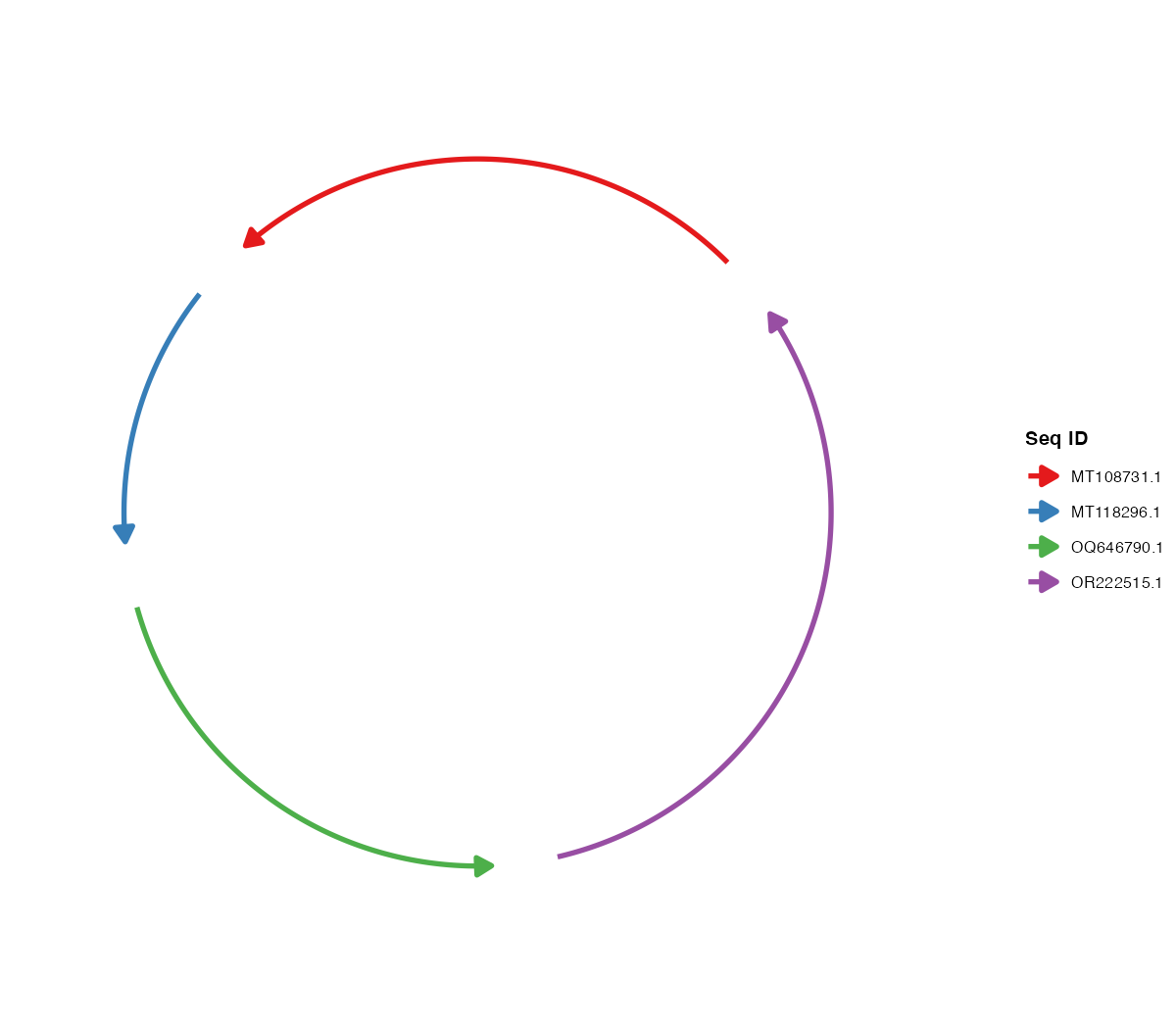
3.4 Add alignment ribbons

ggchord(seq_data_example, ribbon_data_example) +
  geom_seq() + geom_ribbon()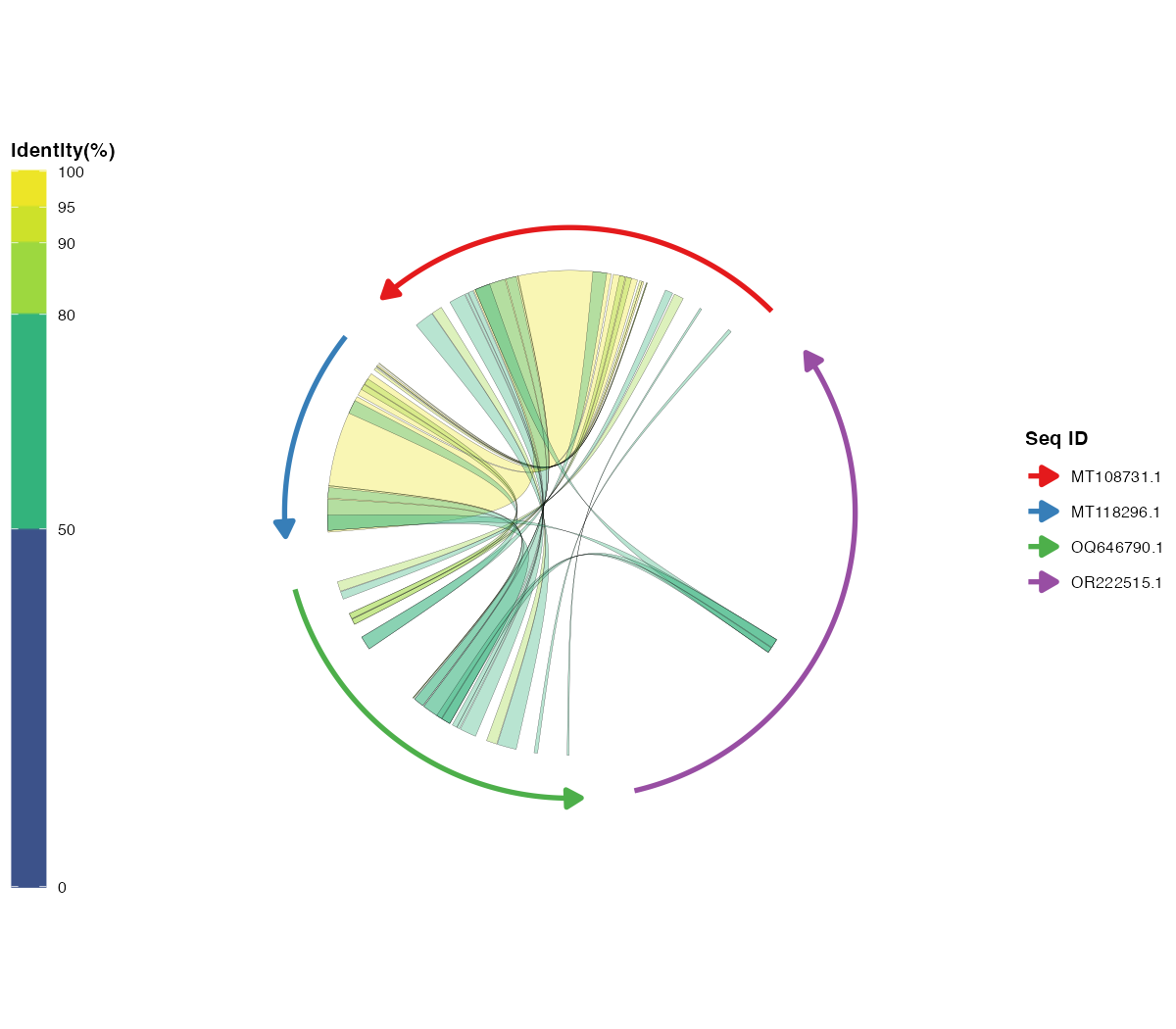

Ribbons coloured by percent identity.

3.5 Add genes and labels

ggchord(seq_data_example, gene_data = gene_data_example) +
  geom_seq() + geom_gene() + geom_gene_label_repel()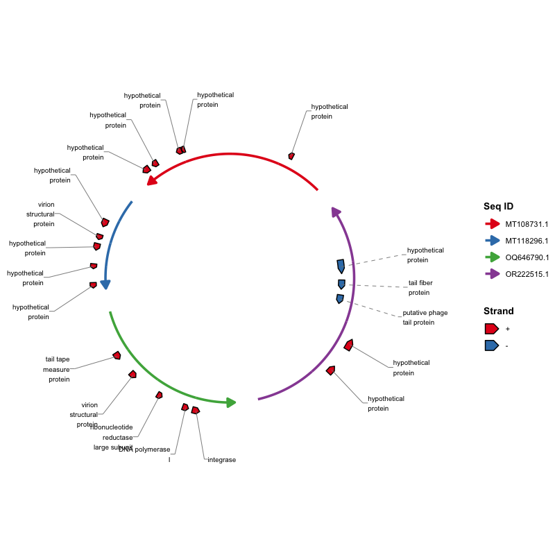

Gene arrows with repelled labels.

Choosing a gene-label layout

geom_gene_label_repel() has three deterministic modes. "aligned" is the default and creates orderly horizontal rows and vertical columns. "radial" keeps text horizontal and uses the nearest collision-free track parallel to the actual sequence curve. "arc" follows the local tangent, flips upside-down text automatically, and only draws a short leader when a label moves away from its first track.

base <- ggchord(seq_data_example, ribbon_data_example, gene_data_example) +
  geom_seq(seq_radius = c(3.3, 2.5, 1.8, 1.25),
           seq_orientation = c(1, -1, 1, -1)) +
  geom_ribbon() + geom_gene()

base + geom_gene_label_repel(gene_label_layout = "aligned")
base + geom_gene_label_repel(gene_label_layout = "radial")
base + geom_gene_label_repel(gene_label_layout = "arc")

Every mode uses the real seq_radius, seq_curvature, seq_gap, seq_orientation, rotation and local curve geometry. The local outside/inside label concepts are informed by SnapGene and Geneious, while ggchord uses generic mode names and an independent implementation. Use geom_gene_label() when manual label rotation or offsets are required.

geom_gene_label() is also the compact fixed-label option. Its v0.10.0 defaults keep text horizontal and outside the chord, then retain labels in input-row order while omitting later collisions. Set gene_label_orientation = "radial" or "tangent", choose gene_label_side = "auto" or "inside", and use gene_label_overlap = "nudge" or "allow" when preserving every requested label is more important than a sparse default. This keeps manual rotation and per-sequence/per-strand offsets in one fixed-label layer rather than adding a separate manual geom.

The broader visual hierarchy draws on Circos, publication-oriented gene arrows in clinker, and annotation collision ideas from DNA Features Viewer. These are design references only; ggchord uses independent palettes, geometry and generic API names.

3.6 Add axes and sequence labels

ggchord(seq_data_example) +
  geom_seq() + geom_axis() + geom_seq_label()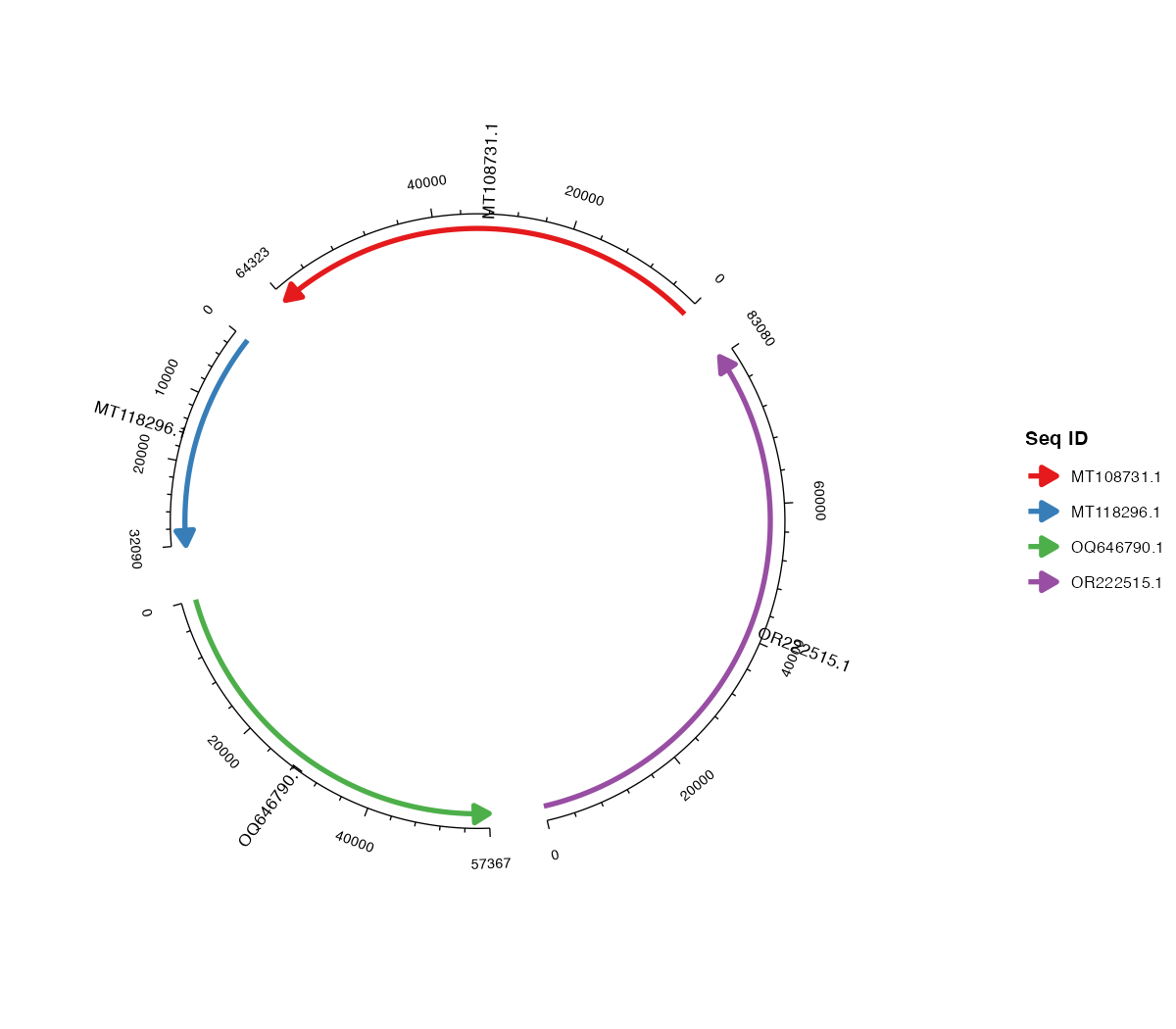

Axes and sequence labels.

3.7 Map numeric ribbon columns and direction

rb_scored <- transform(ribbon_data_example,
                       bitscore = seq_len(nrow(ribbon_data_example)) * 10)

ggchord(seq_data_example, rb_scored) +
  geom_seq() +
  geom_ribbon(ribbon_color_by = "bitscore",
              ribbon_alpha_by = "bitscore",
              ribbon_direction = "linetype")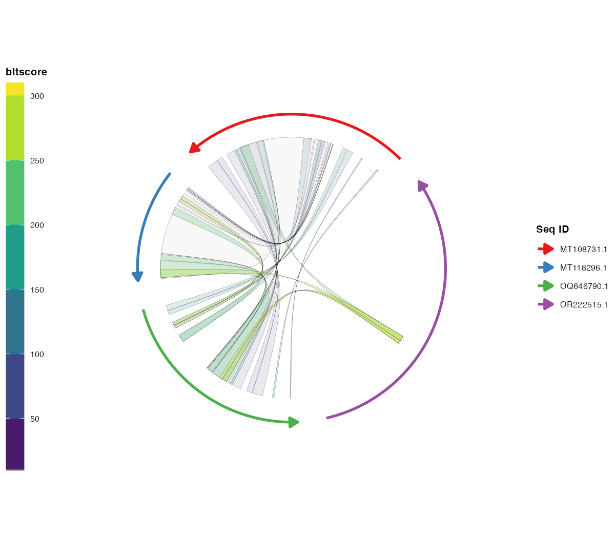

Continuous ribbon fill, alpha and direction mapping.

3.8 Highlight regions and ribbons

regions <- data.frame(seq_id = "MT108731.1",
                      start = 1000, end = 4000, color = "orange")

ggchord(seq_data_example, ribbon_data_example) +
  geom_seq() + geom_ribbon() +
  geom_seq_region(regions = regions) +
  geom_ribbon_highlight(ribbon_ids = 1)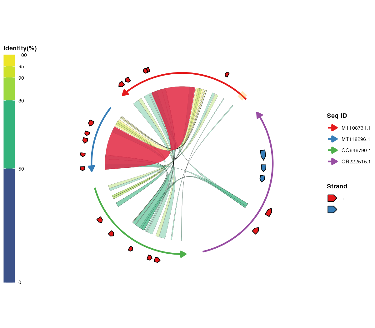

Sequence regions and ribbon highlight.

3.9 Draw generic features

features <- data.frame(seq_id = rep("MT108731.1", 4),
                       start = c(1000, 7000, 13000, 19000),
                       end = c(5000, 11000, 17000, 23000),
                       strand = c("+", "-", "+", "-"),
                       type = c("CDS", "tRNA", "repeat", "promoter"))

ggchord(seq_data_example, ribbon_data_example) +
  geom_seq() + geom_ribbon() +
  geom_feature(aes(feature_shape = type), data = features,
               feature_width = 0.10) +
  scale_feature_shape_manual(values = c(
    CDS = "arrow", tRNA = "block", "repeat" = "chevron",
    promoter = "lollipop"
  ))

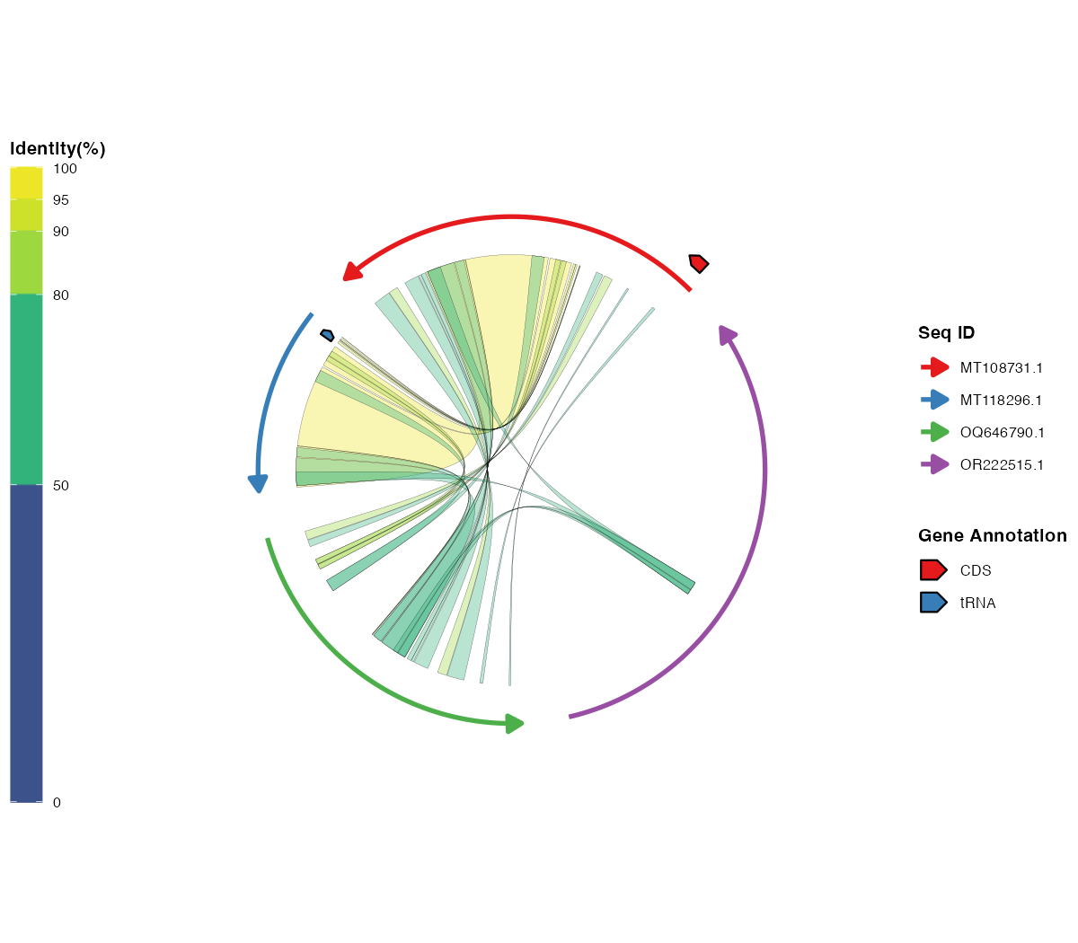
Four feature geometries drawn with geom_feature().

3.10 Apply themes and scales

ggchord(seq_data_example, ribbon_data_example, gene_data_example) +
  geom_seq() + geom_ribbon() + geom_gene() + geom_axis() +
  scale_color_manual(values = c("MT108731.1" = "#E41A1C",
                                "MT118296.1" = "#377EB8",
                                "OQ646790.1" = "#4DAF4A",
                                "OR222515.1" = "#984EA3")) +
  theme(panel.background = element_rect(fill = "grey95"),
        legend.position = "bottom", legend.box = "horizontal")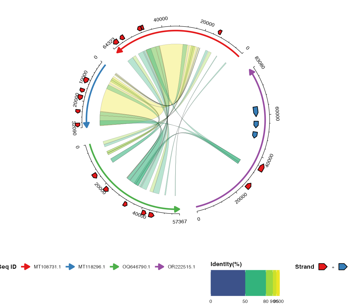

A themed plot with all legends grouped.

3.11 Fine-tuned publication-style plot

ggchord(seq_data_example, ribbon_data_example, gene_data_example,
        title = "ggchord") +
  geom_seq(seq_radius = c(3.3, 2.5, 1.8, 1.25),
           seq_orientation = c(-1, -1, 1, -1),
           seq_colors = c("MT108731.1" = "#E76F51",
                          "MT118296.1" = "#264653",
                          "OQ646790.1" = "#2A9D8F",
                          "OR222515.1" = "#D9A62E")) +
  geom_ribbon(ribbon_alpha = 0.45) +
  geom_gene() +
  geom_gene_label_repel(gene_label_size = 2,
                        gene_label_layout = "aligned") +
  geom_seq_label() +
  geom_axis() +
  theme(plot.background = element_rect(fill = "#FBF9F6", colour = NA),
        panel.background = element_rect(fill = "#FBF9F6", colour = NA))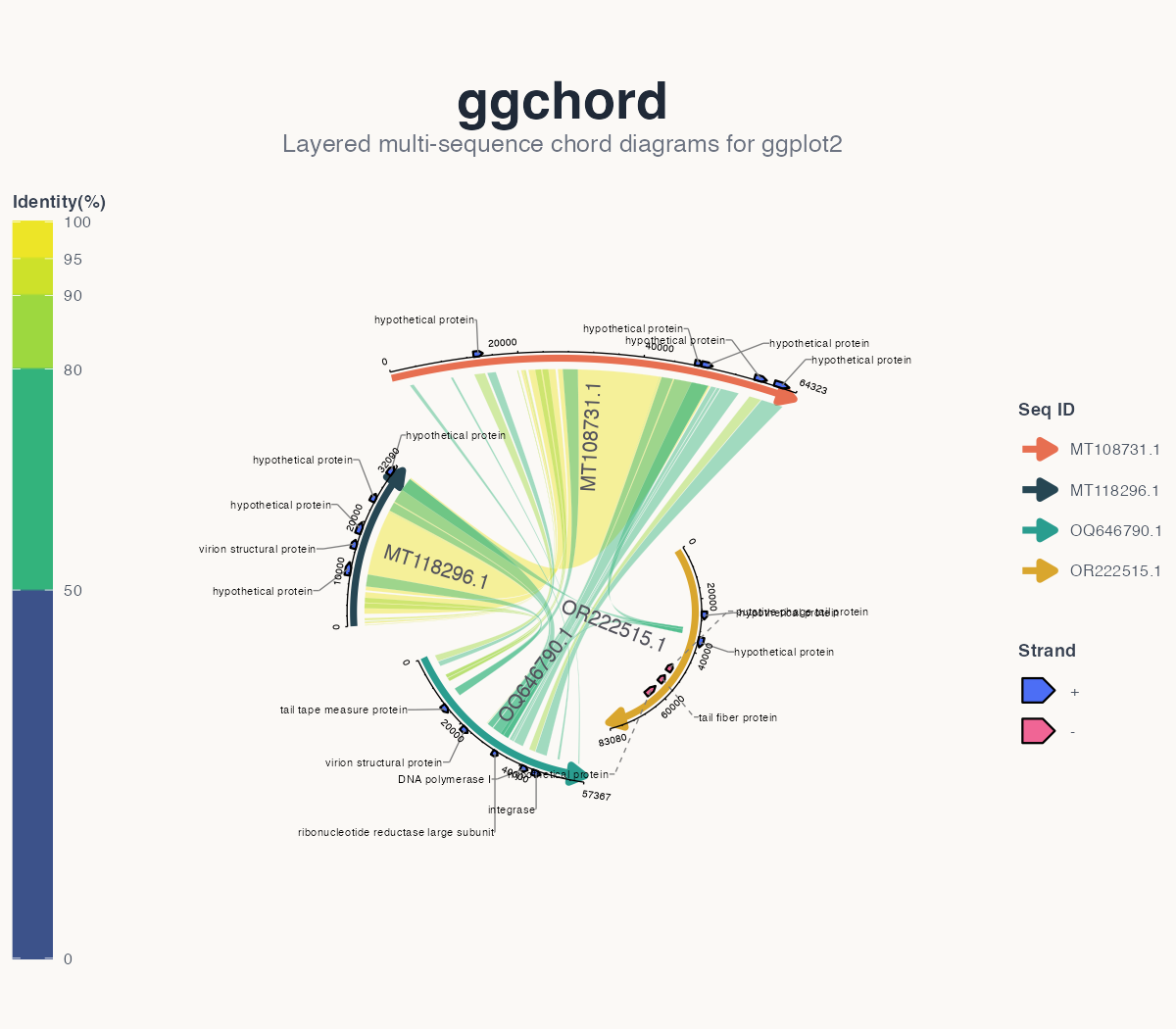

A complete fine-tuned chord diagram.

6. Flexible parameter formats

Sequence-level parameters (seq_radius, seq_gap, axis_label_size, …) accept a single value, an unnamed vector, a vector/list named by sequence ID, a list named by sequence order ("1", "2", …), or an unnamed list. Gene-level parameters of the fixed-position geom_gene_label() layer (gene_label_rotation, gene_offset, …) additionally accept per-strand (+/-) values. The automatic geom_gene_label_repel() modes intentionally manage their own rotation and offsets. All of the following are valid for fixed labels:

# 1. One value for everything
gene_label_rotation = 20

# 2. One value per strand, for every sequence
gene_label_rotation = c("+" = -15, "-" = -45)

# 3. By sequence ID
gene_label_rotation = list(
  "MT118296.1" = c("+" = -15, "-" = -45),
  "OR222515.1" = c("+" = 30, "-" = -30),
  "MT108731.1" = c("+" = 15, "-" = -15),
  "OQ646790.1" = c("+" = 0,  "-" = 0)
)

# 4. By sequence order ("1" = first sequence)
gene_label_rotation = list(
  "1" = c("+" = -15, "-" = -45),
  "2" = c("+" = 30, "-" = -30),
  "3" = c("+" = 15, "-" = -15),
  "4" = c("+" = 0,  "-" = 0)
)

# 5. Unnamed list: follows the sequence order (same as #4)
gene_label_rotation = list(
  c("+" = -15, "-" = -45),
  c("+" = 30, "-" = -30),
  c("+" = 15, "-" = -15),
  c("+" = 0,  "-" = 0)
)

# 6. A length-one list recycles to every sequence
gene_label_rotation = list(20)

7. Layer reference

Layer	Function	Description
Sequence arcs	`geom_seq()`	Draws an arc (or line) for each sequence, with direction arrows
Alignment ribbons	`geom_ribbon()`	Draws colored ribbons from alignment results
Gene arrows	`geom_gene()`	Draws gene/feature arrow polygons
Gene labels	`geom_gene_label()`	Draws gene labels at fixed positions
Automatic gene labels	`geom_gene_label_repel()`	Deterministic aligned, radial or arc layouts with collision-free leaders
Axes	`geom_axis()`	Draws axis lines, major/minor ticks and tick labels
Sequence labels	`geom_seq_label()`	Places sequence names on/outside the arcs

8. Plot interpretation

Sequence arcs — each colored arc is one sequence, with length proportional to the sequence length and arrows showing direction.
Ribbons — colored regions connecting sequences represent aligned/ homologous intervals; color encodes identity, query or subject by default.
Gene arrows — arrow polygons on the sequences; color encodes strand or functional category, with optional labels.
Axes — ticks and numbers outside each arc label sequence positions.