library(ggchord)
library(ggplot2)

data(seq_data_example)
data(ribbon_data_example)
data(gene_data_example)
本教程完整介绍 ggchord 的工作流程:准备输入数据、在 R
中导入文件、 校验与清理数据,以及逐层构建图形。本文对应 v0.9.0
正式版。
1. 前期数据准备
包需要三类输入数据,均为普通数据框。
【必须】序列信息数据(seq_data)
| 列名 | 类型 | 说明 |
|---|---|---|
seq_id |
字符 | 序列唯一标识 |
length |
整数 | 序列长度(必须为正数) |
示例:
| seq_id | length |
|---|---|
| MT108731.1 | 64323 |
| MT118296.1 | 32090 |
| OQ646790.1 | 57367 |
| OR222515.1 | 83080 |
从 FASTA 文件生成该表格的常见方法:
【可选】比对数据(ribbon_data)
每行表示两条序列之间的一个比对片段(列名遵循常见比对工具的输出约定):
| 列名 | 类型 | 说明 |
|---|---|---|
qaccver |
字符 | 查询序列 ID |
saccver |
字符 | 目标序列 ID |
length |
整数 | 比对长度(bp) |
pident |
数值 | 相似度百分比(0–100) |
qstart |
整数 | 查询序列上的起始位置 |
qend |
整数 | 查询序列上的终止位置 |
sstart |
整数 | 目标序列上的起始位置 |
send |
整数 | 目标序列上的终止位置 |
示例行:
| qaccver | saccver | length | pident | qstart | qend | sstart | send |
|---|---|---|---|---|---|---|---|
| MT108731.1 | MT118296.1 | 24856 | 98.612 | 26298 | 51139 | 7121 | 31959 |
| MT108731.1 | MT118296.1 | 4412 | 97.031 | 21513 | 25922 | 2365 | 6772 |
| MT108731.1 | MT118296.1 | 464 | 94.181 | 20691 | 21146 | 1032 | 1495 |
例如,BLAST 的 -outfmt 7
标准输出可以直接解析为该表格:
seqs=("MT108731.1" "MT118296.1" "OQ646790.1" "OR222515.1")
ext="fna"
for ((i=0; i<${#seqs[@]}-1; i++)); do
  for ((j=i+1; j<${#seqs[@]}; j++)); do
    blastn \
      -outfmt '7 qaccver saccver pident length mismatch gapopen qstart qend sstart send evalue bitscore qcovs qlen slen sstrand stitle' \
      -query "examples/fasta/${seqs[$i]}.${ext}" \
      -subject "examples/fasta/${seqs[$j]}.${ext}" \
      -out "examples/blastn/${seqs[$i]}__${seqs[$j]}.o7"
  done
done【可选】基因数据(gene_data)
每行表示一条序列上的一个基因(或其他特征):
| 列名 | 类型 | 说明 |
|---|---|---|
seq_id |
字符 | 基因所属序列 ID |
start |
整数 | 基因起始位置 |
end |
整数 | 基因终止位置 |
strand |
字符 | 链方向(+ 或 -) |
anno |
字符 | 基因注释 / 功能类别 |
示例行:
| seq_id | start | end | strand | anno |
|---|---|---|---|---|
| MT108731.1 | 60709 | 63087 | + | hypothetical protein |
| MT118296.1 | 14628 | 16301 | + | virion structural protein |
| OQ646790.1 | 43765 | 46140 | + | integrase |
| OQ646790.1 | 13194 | 15551 | + | tail tape measure protein |
例如,可由 GFF3 文件转换得到:
library(tidyverse)
gff3FilesPath <- list.files(path = "examples/gff3", pattern = "\\.gff3$", full.names = TRUE)
gff3Table <- map_df(gff3FilesPath, ~read_tsv(.x, show_col_types = F, comment = "#",
  col_names = F) %>% set_names(c("seq_id", "source", "type", "start", "end",
  "score", "strand", "phase", "attributes")))
geneTrackTable <- gff3Table %>%
  filter(type == "CDS") %>%
  mutate(anno = str_extract(attributes, "(?<=product=)[^;]+(?=;)")) %>%
  select(seq_id, start, end, strand, anno)
write_tsv(geneTrackTable, "examples/gene_track.tsv")
2. 在 R 中导入 FASTA / BLAST / GFF3 数据
外部命令行工具(BLAST、seqkit 等)通常用于准备数据,但它们产出的文件 也可以直接用包内置的导入助手在 R 中读取,从而把「在 R 外准备数据」与 「在 R 中导入并绘图」两个步骤清晰分开:
library(ggchord)

# FASTA -> seq_data(读取并合并全部示例 FASTA 文件)
seq_data <- invisible(read_fasta_lengths(files = "examples/fasta/*.fna"))

# BLAST -outfmt 6/7 表格输出 -> ribbon_data(12 或 17 列自动识别)
ribbon_data <- invisible(read_blast(files = "examples/blastn/*.o7"))

# GFF3 -> gene_data(默认取 CDS;anno 从 product/Name/... 属性提取)
gene_data <- invisible(read_gff3(files = "examples/gff3/*.gff3"))

ggchord(seq_data, ribbon_data, gene_data) +
  geom_seq() + geom_ribbon() + geom_gene()
read_blast()
保留有用的额外列(evalue、bitscore、qcovs、qlen、
slen、sstrand、stitle);read_gff3()
保留 type、source、
score、phase、attributes;read_fasta_lengths()
可通过 header_delim = "|" 拆分 NCBI 风格标题。
3. 使用教程:从数据到弦图
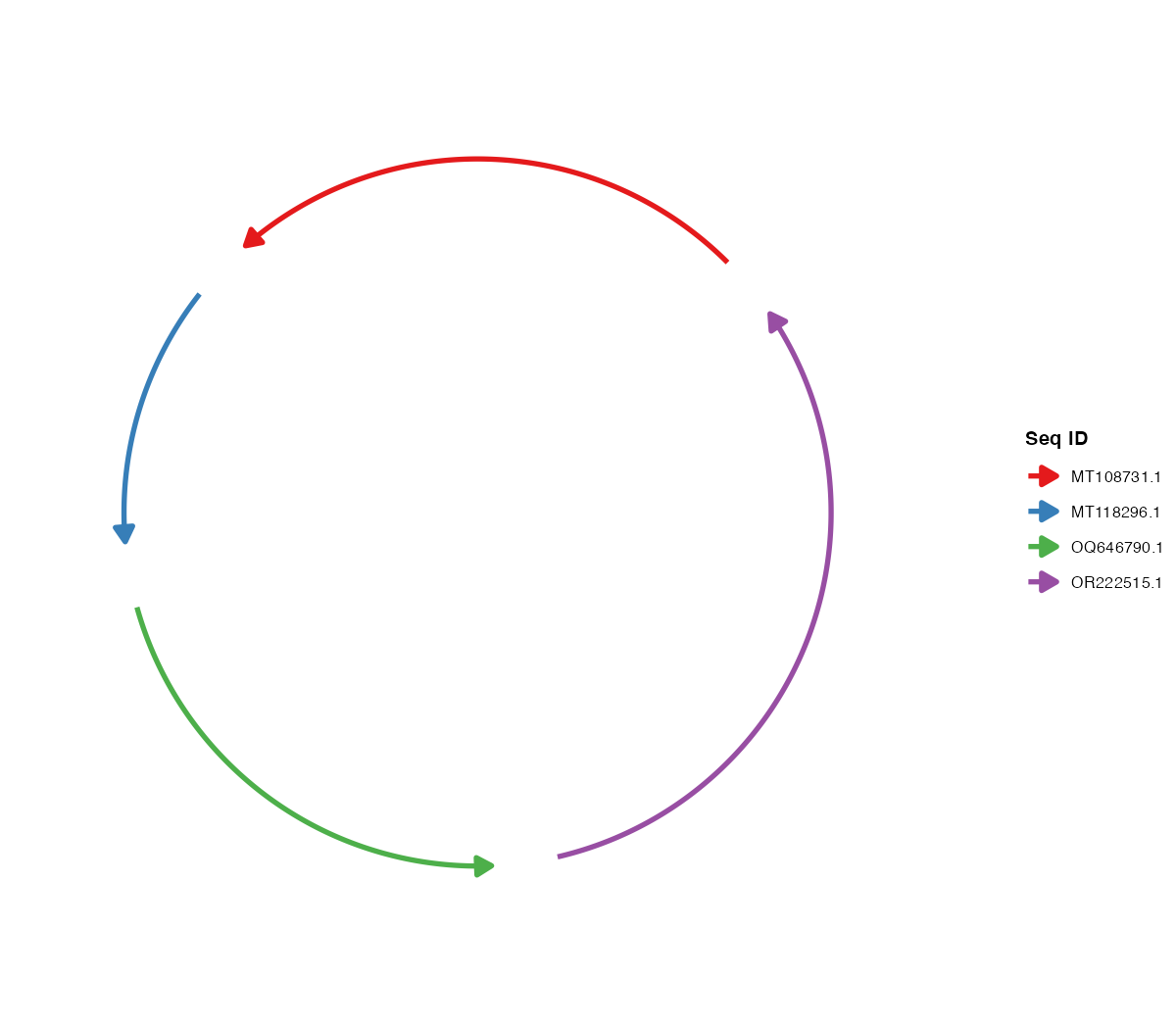
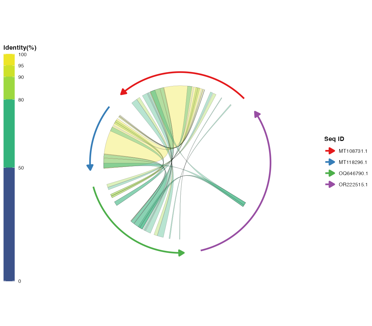
本节把准备好的数据逐步变成完整弦图。每一步都给出简短示例与对应图片。
3.1 校验并清理数据
data(seq_data_example)
data(ribbon_data_example)
data(gene_data_example)

validate_ggchord_data(seq_data_example, ribbon_data_example, gene_data_example)

clean_ggchord_data(seq_data_example, ribbon_data_example, gene_data_example,
                   unknown_id = "drop", out_of_range = "clip",
                   reversed_interval = "sort", invalid_pident = "clip")
ggchord()
默认也会执行校验(validate = "warn")。用
"error" 可在严重问题时停止,用 "none"
可跳过诊断以处理大数据。
3.2 筛选并合并 Ribbon
kept <- filter_ggchord_ribbons(ribbon_data_example, min_pident = 90,
                               drop_self_links = TRUE,
                               sort_by = "pident")
dedup <- deduplicate_ggchord_ribbons(kept$data, by = "exact",
                                     keep = "best_pident")
merged <- merge_ggchord_ribbons(dedup$data, max_gap = 0)
返回的 $data 可直接传入 ggchord()。
3.5 加入基因与标签
ggchord(seq_data_example, gene_data = gene_data_example) +
geom_seq() + geom_gene() + geom_gene_label_repel()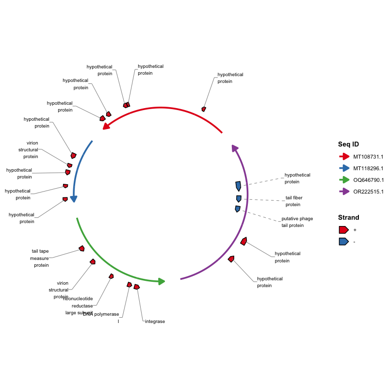
带防重叠标签的基因箭头。
选择基因标签布局
geom_gene_label_repel() 提供三种确定性模式。默认
"aligned" 将水平文字
排成规则的行和垂直列;"radial"
保持文字水平,并沿真实序列曲线选择最近的
无冲突平行轨道;"arc"
沿局部切线旋转文字、自动翻转倒置文字,并且只在
标签离开第一轨道后绘制短指示线。
base <- ggchord(seq_data_example, ribbon_data_example, gene_data_example) +
geom_seq(seq_radius = c(3.3, 2.5, 1.8, 1.25),
seq_orientation = c(1, -1, 1, -1)) +
geom_ribbon() + geom_gene()
base + geom_gene_label_repel(gene_label_layout = "aligned")
base + geom_gene_label_repel(gene_label_layout = "radial")
base + geom_gene_label_repel(gene_label_layout = "arc")三种模式都会使用实际的
seq_radius、seq_curvature、seq_gap、
seq_orientation、旋转和局部曲线几何。局部外侧/内侧标签理念借鉴了
SnapGene
与 Geneious,但
ggchord 使用通用模式名和独立实现。如需手工旋转或偏移,请使用
geom_gene_label()。
geom_gene_label() 也是紧凑的固定标签方案。v0.10.0
默认将文字水平放在
弦图外侧,按输入行顺序保留标签并省略后续冲突项。可以用
gene_label_orientation = "radial" 或 "tangent"
改变文字方向,用 gene_label_side = "auto" 或
"inside" 选择侧向,并用
gene_label_overlap = "nudge" 或 "allow"
优先保留全部文字。手工旋转和逐序列/
逐链偏移仍集中在这一个固定标签图层中,不新增重复的手动 geom。
整体信息层级还借鉴了 Circos、 clinker 的发表级基因箭头, 以及 DNA Features Viewer 的注释冲突处理思路。 这些只是设计原则参考,ggchord 使用独立的配色、几何和通用 API 名称。
3.7 映射数值列与 Ribbon 方向
rb_scored <- transform(ribbon_data_example,
bitscore = seq_len(nrow(ribbon_data_example)) * 10)
ggchord(seq_data_example, rb_scored) +
geom_seq() +
geom_ribbon(ribbon_color_by = "bitscore",
ribbon_alpha_by = "bitscore",
ribbon_direction = "linetype")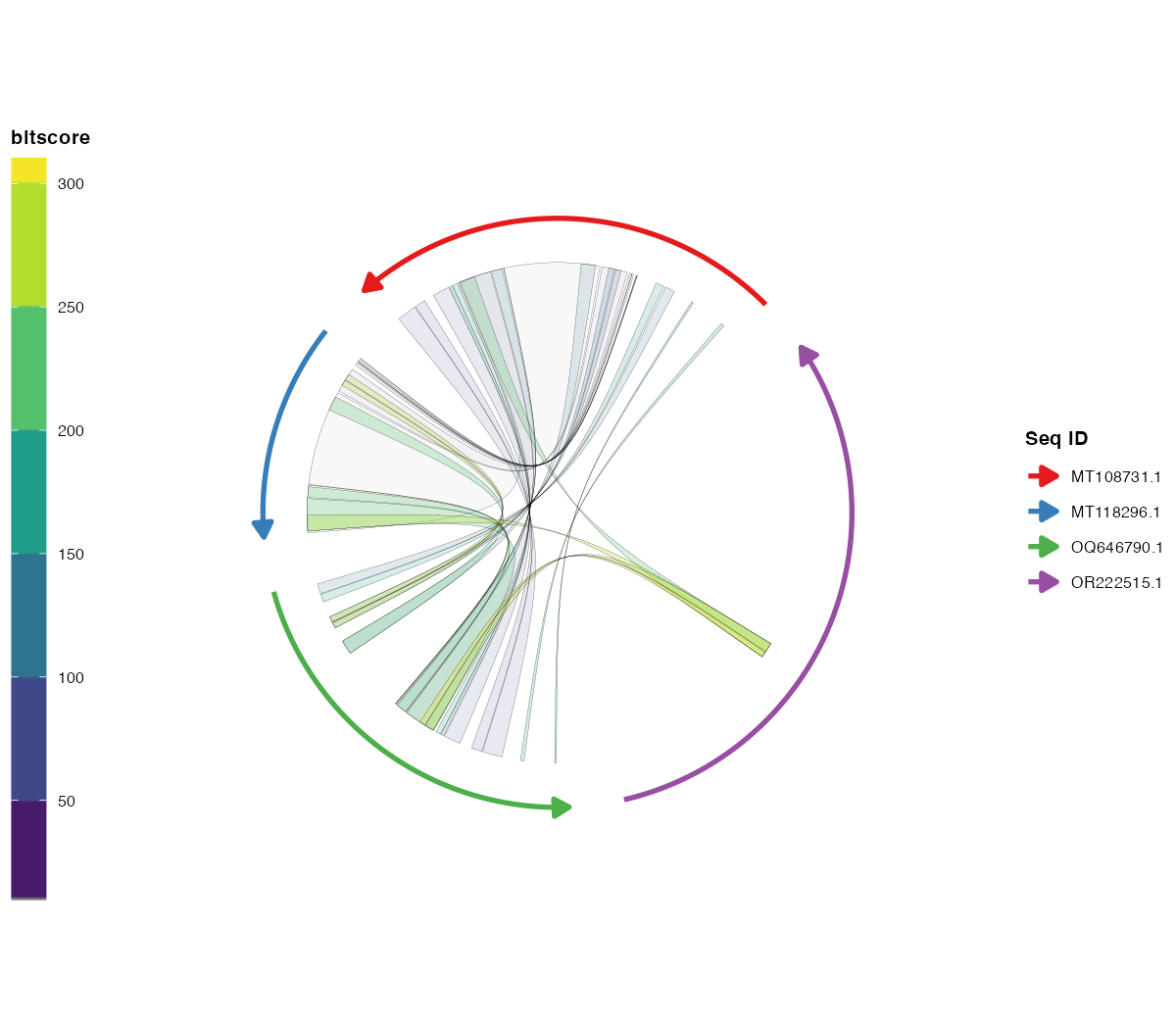
连续填充、透明度与方向映射。
3.8 高亮区间与连接带
regions <- data.frame(seq_id = "MT108731.1",
start = 1000, end = 4000, color = "orange")
ggchord(seq_data_example, ribbon_data_example) +
geom_seq() + geom_ribbon() +
geom_seq_region(regions = regions) +
geom_ribbon_highlight(ribbon_ids = 1)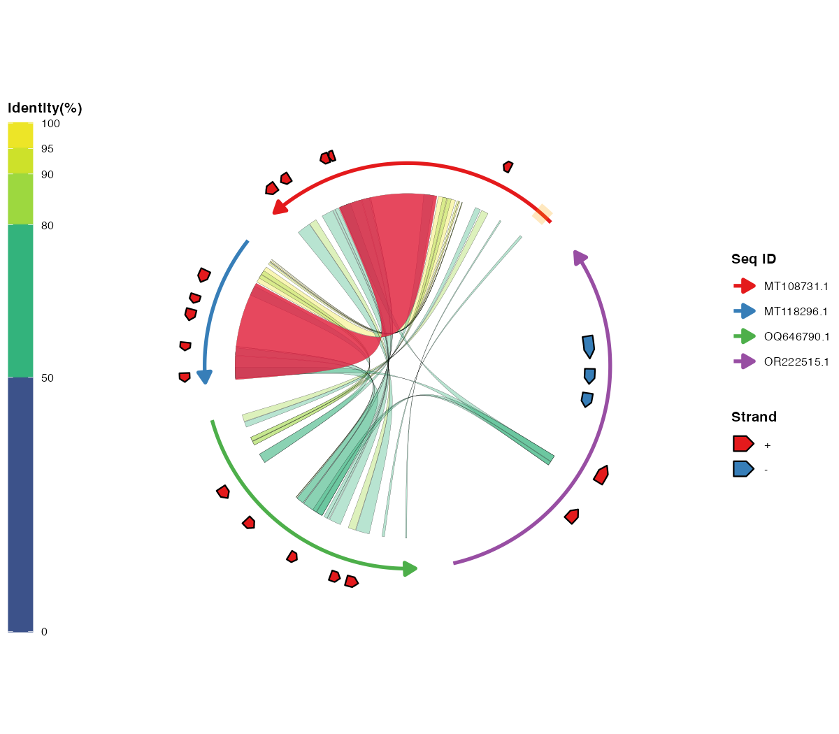
序列区间与连接带高亮。
3.9 绘制通用 feature
features <- data.frame(seq_id = rep("MT108731.1", 4),
                       start = c(1000, 7000, 13000, 19000),
                       end = c(5000, 11000, 17000, 23000),
                       strand = c("+", "-", "+", "-"),
                       type = c("CDS", "tRNA", "repeat", "promoter"))

ggchord(seq_data_example, ribbon_data_example) +
  geom_seq() + geom_ribbon() +
  geom_feature(aes(feature_shape = type), data = features,
               feature_width = 0.10) +
  scale_feature_shape_manual(values = c(
    CDS = "arrow", tRNA = "block", "repeat" = "chevron",
    promoter = "lollipop"
  ))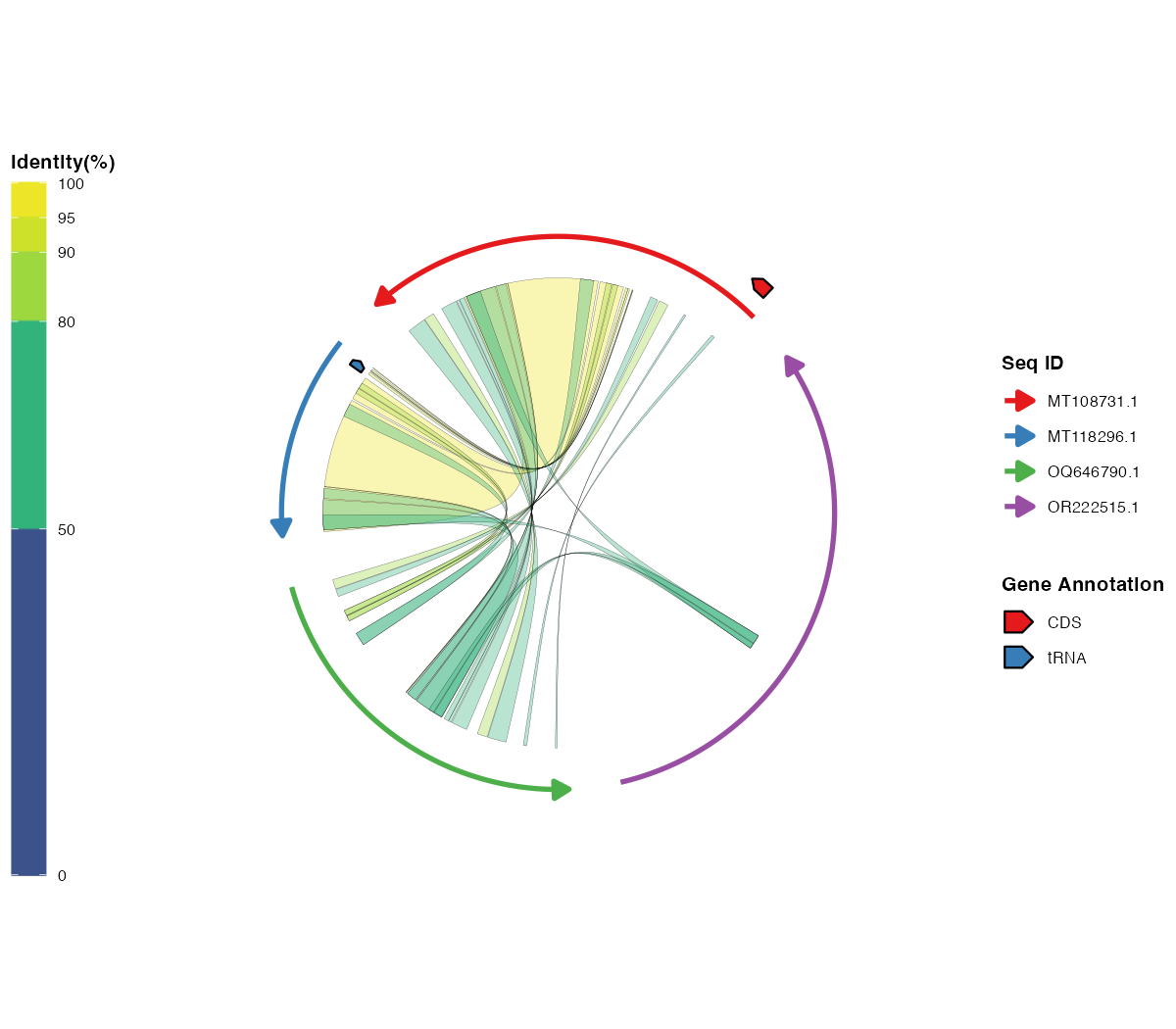
用 geom_feature() 绘制的四种 feature 几何。
3.10 应用主题与 scale
ggchord(seq_data_example, ribbon_data_example, gene_data_example) +
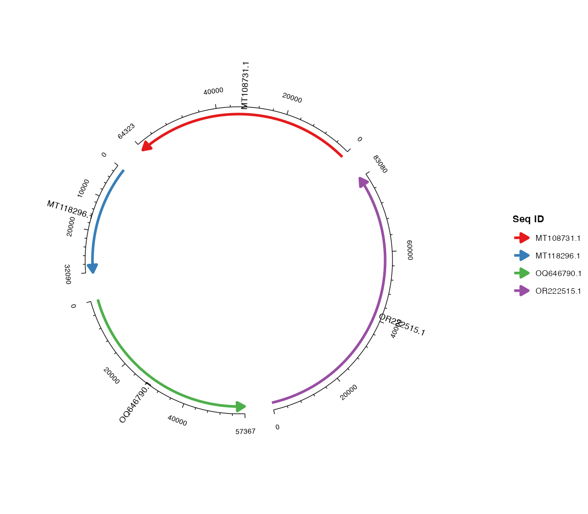
  geom_seq() + geom_ribbon() + geom_gene() + geom_axis() +
  scale_color_manual(values = c("MT108731.1" = "#E41A1C",
                                "MT118296.1" = "#377EB8",
                                "OQ646790.1" = "#4DAF4A",
                                "OR222515.1" = "#984EA3")) +
  theme(panel.background = element_rect(fill = "grey95"),
        legend.position = "bottom", legend.box = "horizontal")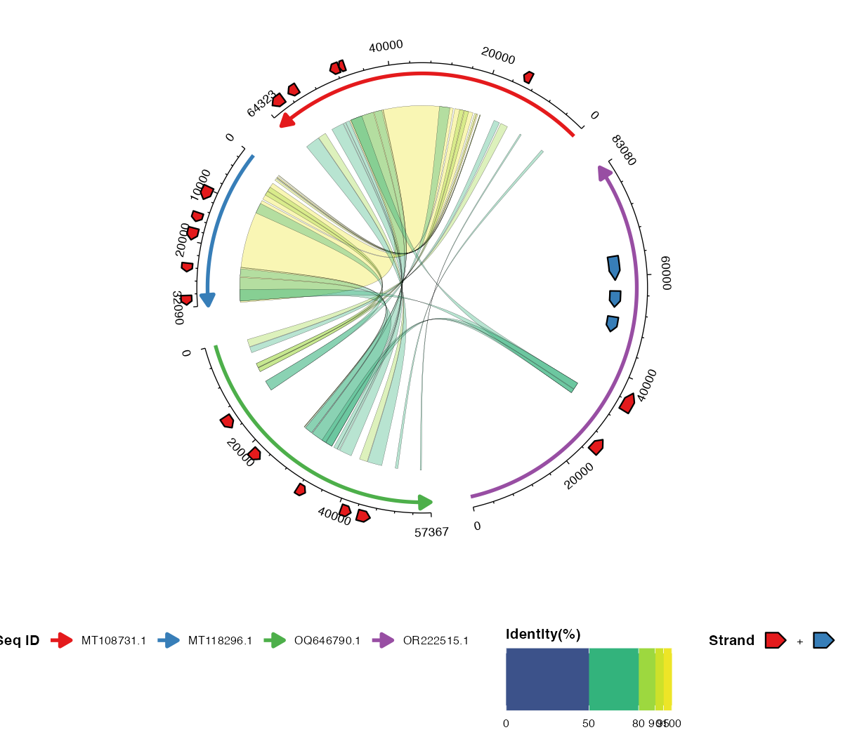
统一图例的主题化图形。
3.11 发表级精细控制
ggchord(seq_data_example, ribbon_data_example, gene_data_example,
        title = "ggchord") +
  geom_seq(seq_radius = c(3.3, 2.5, 1.8, 1.25),
           seq_orientation = c(-1, -1, 1, -1),
           seq_colors = c("MT108731.1" = "#E76F51",
                          "MT118296.1" = "#264653",
                          "OQ646790.1" = "#2A9D8F",
                          "OR222515.1" = "#D9A62E")) +
  geom_ribbon(ribbon_alpha = 0.45) +
  geom_gene() +
  geom_gene_label_repel(gene_label_size = 2,
                        gene_label_layout = "aligned") +
  geom_seq_label() +
  geom_axis() +
  theme(plot.background = element_rect(fill = "#FBF9F6", colour = NA),
        panel.background = element_rect(fill = "#FBF9F6", colour = NA))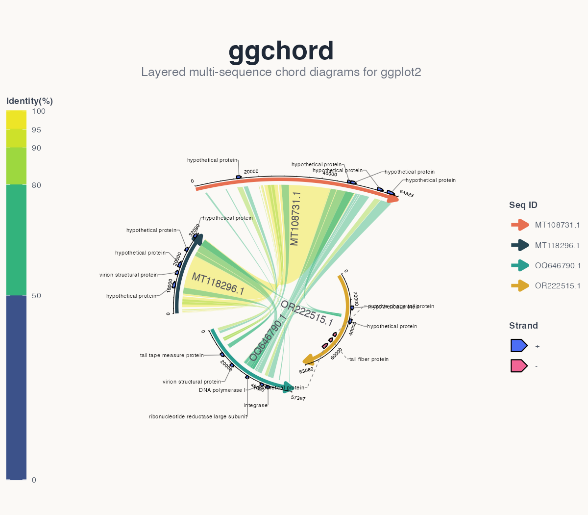
精细控制下的完整弦图。
6. 灵活的参数格式
序列级参数(seq_radius、seq_gap、axis_label_size
等)支持单值、无名向量、按序列 ID
命名的向量/列表、按序列顺序命名的列表("1"、"2"…)或无名列表。固定位置图层
geom_gene_label()
的基因级参数(gene_label_rotation、gene_offset
等)还额外支持按链方向(+/-)指定;自动布局
geom_gene_label_repel()
会自行管理旋转与偏移。以下写法适用于固定标签:
# 1. 全部使用同一个值
gene_label_rotation = 20

# 2. 每条序列按链方向分别指定
gene_label_rotation = c("+" = -15, "-" = -45)

# 3. 按序列 ID 名称指定
gene_label_rotation = list(
  "MT118296.1" = c("+" = -15, "-" = -45),
  "OR222515.1" = c("+" = 30, "-" = -30),
  "MT108731.1" = c("+" = 15, "-" = -15),
  "OQ646790.1" = c("+" = 0,  "-" = 0)
)

# 4. 按序列顺序指定("1" 表示第一条序列)
gene_label_rotation = list(
  "1" = c("+" = -15, "-" = -45),
  "2" = c("+" = 30, "-" = -30),
  "3" = c("+" = 15, "-" = -15),
  "4" = c("+" = 0,  "-" = 0)
)

# 5. 无名列表:按序列顺序(与 #4 等价)
gene_label_rotation = list(
  c("+" = -15, "-" = -45),
  c("+" = 30, "-" = -30),
  c("+" = 15, "-" = -15),
  c("+" = 0,  "-" = 0)
)

# 6. 长度为一的列表会循环应用到每条序列
gene_label_rotation = list(20)
7. 图层参考
| 图层 | 函数 | 说明 |
|---|---|---|
| 序列弧线 | geom_seq() |
为每条序列绘制弧线(或直线),含方向箭头 |
| 比对连接带 | geom_ribbon() |
根据比对结果绘制彩色连接带 |
| 基因箭头 | geom_gene() |
绘制基因/特征箭头多边形 |
| 基因标签 | geom_gene_label() |
在固定位置绘制基因标签 |
| 自动基因标签 | geom_gene_label_repel() |
确定性的 aligned、radial 或 arc 布局,并自动避免标签和指示线冲突 |
| 坐标轴 | geom_axis() |
绘制坐标轴线、主/次刻度与刻度标签 |
| 序列标签 | geom_seq_label() |
在弧线内侧/外侧放置序列名称 |
8. 图形解读
- 序列弧线——每条彩色弧线代表一条序列,长度按比例映射,箭头表示方向。
- 连接带——连接序列之间的彩色区域代表比对/同源区间;默认颜色编码相似度、查询或目标序列。
- 基因箭头——绘制在序列上的箭头多边形;颜色编码链方向或功能类别,可选标签。
- 坐标轴——每条弧线外侧的刻度与数字标注序列位置。